Random Averaging

Module information
Modules	BESA Research Basic or higher
Version	5.2 or higher

Abstract

The idea of this tutorial is to provide a procedure for random averaging of row data containing triggers. The advantage of random averaging is that the result is not only one average over the trials but many different averages of the same data with different choice of trials and these averages can be statistically analyzed in order to get a statistically verified differences between the signal before and the signal after the trigger point. This can be applied e.g. in the source space and it can be used to determine brain regions with a statistically significant activity against baseline. All steps in this article are demonstrated on a file from the examples of BESA Research - "S1.cnt".

Export the single trial data in simple binary file format

Load from the examples of BESA Research the file "S1.cnt" in the folder "ERP-Auditory-Intensity". After the file was loaded select menu "File → Export...". The "Export data" dialog opens (see Figure 1).

In that dialog select "Epochs around triggers" in the section "Data to export". The two buttons "Interval..." and "Triggers..." become active. Then click on "Interval..." to set appropriate values for the time interval around the trigger and after that click on "Triggers..." in order to select trigger for the random averaging. Please make sure to select only one trigger (see Figure 2) else the generated random averages will contain mixed data from all selected triggers. In the "Export data"-dialog click "OK" to export the data.

• 

  

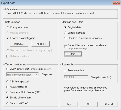  Figure 1 The "Export data"-dialog
• 

  

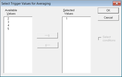  Figure 2 "Select trigger"-dialog

Use the external tool BesaRandomAveraging.exe to generate the random averages

There exists a tool called "BesaRandomAveraging.exe" which is designed for that to load the exported single trial data and to generate random averages. This tool is based on a Python script called "BesaRandomAveraging.py" which is open source. Both, the source and the binary can be downloaded from here [1] . The usage of the tool is as follows:

BesaRandomAveraging.exe -f <inputfile> ...
-n <number of averages> -t <number of trials>

where <inputfile> is the absolute path (directory + filename) to the file containing the exported single trial data, <number of averages> is the number of random averages to create and <number of trials used for averaging> is the number of trials which are selected for each average.

Example:

BesaRandomAveraging.exe -f N:\\Python\\data\\ ...
S1-export.dat -n 20 -t 50

This command line will generate 20 different averages using sample of 50 trials for every average. It is possible to start the tool from the DOS prompt or directly from BESA Research (see Figure 3) using the following batch command:

GENRunProcess(...)

Figure 3 Dialog for the batch command "GENRunProcess(...)"

Perform source analysis on the averages

Once the random averages are created we want to perform source analysis on them. For this purpose we are going to use batch in order to save time. The following batch can be used for the source analysis using LORETA:

MAINFilter(LC:0.50-6dB-f,HC:45.00-24dB-z,NF:off,BP:off)
MAINMarkBlock(WholeSegment,-,1,SendToSA)
SAimageLORETA(NoImageWeights,ForceRecompute)
SAimageExport(%basename%_LORETA.dat,All,ASCII,-)
SAexit()

The first line sets the filter, the second marks the entire interval and sends it to the source analysis module, the third computes LORETA over the entire interval, the fourth exports the LORETA results as an ASCII-file and the last just exits the source analysis module. Now we have the LORETA results for the entire time interval, however, we need additional results to compare with. This could be either a control condition or LORETA results from the baseline interval. In this tutorial we choose to use the baseline interval. In that case we should use another batch script which is very similar to the previous one in order to calculate LORETA only for the baseline interval:

MAINFilter(LC:0.50-6dB-f,HC:45.00-24dB-z,NF:off,BP:off)
MAINMarkBlock(WholeSegment,-,1,SendToSA)
SAfitInterval(-100,0,FitInterval)
SAimageLORETA(NoImageWeights,ForceRecompute)
SAimageExport(%basename%_LORETA.dat,All,ASCII,-)
SAexit()

The only difference with respect to the previous script is the command SAfitInterval(-100,0,FitInterval) which sets only the baseline interval [-100 0] for the source localization.

Calculate root-mean-square (RMS) over the time points in the baseline in order to get only one source image for the baseline interval

Now the LORETA source reconstruction files are generated and we want to compare the evoked response and the response in the baseline in order to get the regions in the brain which are statistically significant. For this purpose we have to choose how to do that. One possible problem is that the baseline interval is not necessarily exactly as long as the interval containing the evoked response of interest. Consequently, it is more convenient to use baseline interval which is as long as we need it. In order to achieve that we calculate the root-mean-square over the time for LORETA images calculated in the baseline interval. In that way we get for every random average one LORETA image representing the localization results for the baseline. After that we can stretch this image to as many time points as we need and save the 4D matrix in an ASCII file. These steps can be performed with a Matlab script:

%% create constant baseline
 
addpath('N:\BESA_MATLAB\BesaIO\besa_matlab_readers')
addpath('N:\BESA_MATLAB\BesaIO\ersam2besa')
 
DataPathSignal = 'N:\Python\data\LoretaData';
DataPathBaseline = 'N:\Python\data\Baseline';
DataPathConstBaseline = 'N:\Python\data\ConstantBaseline';
 
FirstTimeSample = -100.0; % ms
TimeStep = 4; % ms
ImageMethod = 'Standard LORETA';
 
FileNames = ...
    {'S1-export_new15_LORETA.dat',  'S1-export_new4_LORETA.dat', ... 
    'S1-export_new16_LORETA.dat',  'S1-export_new5_LORETA.dat', ...  
    'S1-export_new0_LORETA.dat',   'S1-export_new17_LORETA.dat', ... 
    'S1-export_new6_LORETA.dat',   'S1-export_new10_LORETA.dat', ... 
    'S1-export_new18_LORETA.dat',  'S1-export_new7_LORETA.dat', ...  
    'S1-export_new11_LORETA.dat',  'S1-export_new19_LORETA.dat', ... 
    'S1-export_new8_LORETA.dat',   'S1-export_new12_LORETA.dat', ... 
    'S1-export_new1_LORETA.dat',   'S1-export_new9_LORETA.dat',  ... 
    'S1-export_new13_LORETA.dat',  'S1-export_new2_LORETA.dat',  ... 
    'S1-export_new14_LORETA.dat',  'S1-export_new3_LORETA.dat'};
 
NumFiles = length(FileNames);
 
for f=1:NumFiles
 
    CurrFilename = FileNames{f};
 
    CompletePathBaseline = fullfile(DataPathBaseline, CurrFilename);
    CompletePathSignal = fullfile(DataPathSignal, CurrFilename);
    ConstantBaselineData = fullfile(DataPathConstBaseline, CurrFilename);
 
    BaselineData = readBESAimage(CompletePathBaseline);
    SignalData = readBESAimage(CompletePathSignal);
 
    NumTimeSamples = size(SignalData.Data, 4);
 
    % Average baseline over time
%     data4 = squeeze(mean(BaselineData.Data, 4));
    data4 = squeeze(rms(BaselineData.Data, 4));
    data5 = repmat(data4, [1 1 1 NumTimeSamples]);
    data6 = permute(data5, [4 1 2 3]);
 
    besa_save4DimageData(ConstantBaselineData, data6, ...
        min(SignalData.Coordinates.X), min(SignalData.Coordinates.Y), ...
        min(SignalData.Coordinates.Z), max(SignalData.Coordinates.X), ...
        max(SignalData.Coordinates.Y), max(SignalData.Coordinates.Z), ...
        length(SignalData.Coordinates.X), length(SignalData.Coordinates.Y), ...
        length(SignalData.Coordinates.Z), ImageMethod, ...
        FirstTimeSample, TimeStep)
 
end

The external functions used in this script are part of our open source tools "besa_matlab_readers" and "ersam2besa" which can be downloaded from our ftp-server here: [2].

Perform statistical comparison with the results

After all source reconstruction files were generated it remains to compare the evoked responses against the baseline responses. This can be done with BESA Statistics using either paired t-test or within ANOVA projects.