Seed dipole solutions from cortical images

Module information
Modules	BESA Research Basic or higher
Version	5.2 or higher

BESA initially was designed to compute comprehensive dipole solution of so called inverse solution. With the advance of neruoinformatics we also incorporated many popular volumetric solutions (i.e. LORETA) and our own algorithms (like CLARA). Since release 6.1 of BESA Research cortical solutions (i.e. Cortical LORETA) are also available. As always both inverse problem solutions (dipole and 3D Imaging methods) has some pros and cons. For example during dipole analysis, number of dipoles has to be assumed by the user. 3D Imaging methods does not need such assumption, but not provide full information of electrical sources (orientation and waveform of the source).

To overcome such limitation, there is possibility to seed dipole solutions from 3D and cortical images.

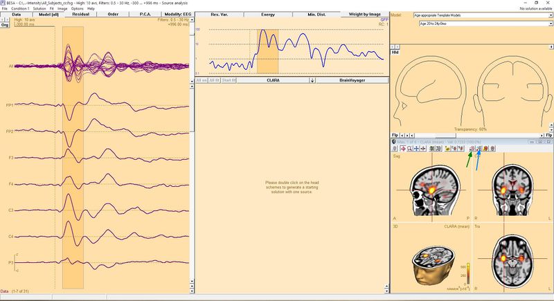
When you have a source analysis window open and you did used 3D Imaging source analysis of your choice you might end with something similar to this (CLARA algorithm was used in this example):

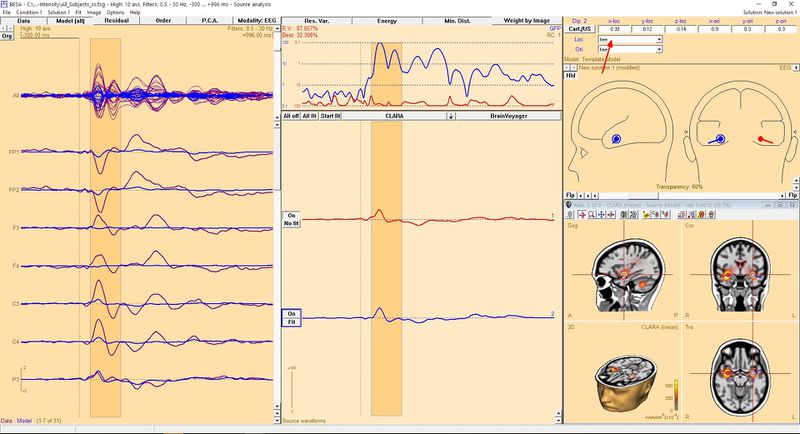
To seed a dipole in exact place where the source is, press button named "Switch to next grid maximum" (button with little M letter, indicated with green arrow in the image). This will place a crosshair in exact place of source maximum designed by 3D image algorithm. You can press this button once again if you want to switch to next maximum. If you press button while holding Ctrl key, you go to previous maximum. When you find the place where you want to seed dipole just press button with dipole on it (indicated with blue arrow in Figure above). Of course you can repeat these steps to seed more than one dipole. For example in presented case you might want to seed two dipoles, as CLARA indicates two potential sources (in both hemispheres in temporal lobe). After doing this we get following result:

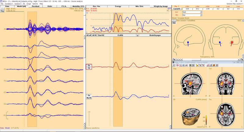
To get better approximation of dipoles, we should fit them. Since the dipoles was placed on the basis of 3D image, good idea is to keep their location in the original position (to maintain visual connection between both solutions). So for each dipole we need to change location from "free" to "fixed" by selecting it from the list indicated with red arrow. You can switch between dipoles just by clicking on it. When this is done you can fit all dipoles to data. Press "All fit" button in the middle window to select all dipoles. Now press "Start fit". The result of such operation is presented below. please note that the waveforms and orientation has changed but location not.