Difference between revisions of "Source Analysis 3D Imaging"
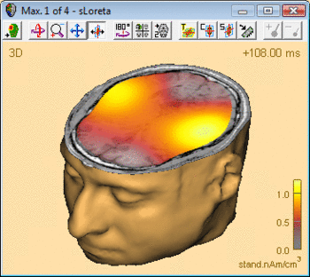
(→sLORETA) |
|||
| (37 intermediate revisions by 4 users not shown) | |||
| Line 2: | Line 2: | ||
|title = Module information | |title = Module information | ||
|module = BESA Research Standard or higher | |module = BESA Research Standard or higher | ||
| − | |version = 6.1 or higher | + | |version = BESA Research 6.1 or higher |
}} | }} | ||
| Line 91: | Line 91: | ||
'''Applying the Beamformer''' | '''Applying the Beamformer''' | ||
| − | This chapter illustrates the usage of the BESA beamformer. The displayed figures are generated using the file <span style="color:#ff9c00;">''''Examples/Learn-by-Simulations/AC-Coherence/AC-Osc20.foc''''</span> (see BESA Tutorial | + | This chapter illustrates the usage of the BESA beamformer. The displayed figures are generated using the file <span style="color:#ff9c00;">''''Examples/Learn-by-Simulations/AC-Coherence/AC-Osc20.foc''''</span> (see BESA Tutorial 12: "''Time-frequency analysis, Connectivity analysis, and Beamforming''"). |
| Line 101: | Line 101: | ||
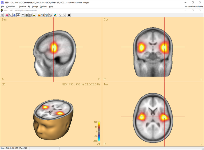
| − | [[Image:SA 3Dimaging (5). | + | [[Image:SA 3Dimaging (5).png|700px|thumb|c|none|Beamformer image after starting the computation in the Time-Frequency window. A bilateral pair of sources in the auditory cortex accounts for the highly correlated oscillatory induced activity. Only the bilateral beamformer manages to separate these activities; a traditional single-source beamformer would merge the two sources into one image maximum in the head center instead.]] |
| − | + | ||
| − | + | ||
| Line 111: | Line 109: | ||
| − | [[Image:SA 3Dimaging (6). | + | [[Image:SA 3Dimaging (6).png|700px|thumb|c|none|Source Analysis window with beamformer image. The two sources have been added using the ''<span style="color:#3366ff;">'''Switch to'''</span>'' ''<span style="color:#3366ff;">'''Maximum'''</span>'' and ''<span style="color:#3366ff;">'''Add Source '''</span>''toolbar buttons (see below). Source waveforms are computed from the displayed averaged data. Therefore, they do not represent the activity displayed in the beamformer image, which in this simulation example is induced (i.e. not phase-locked to the trigger)!]] |
| − | + | ||
| − | + | ||
| Line 119: | Line 115: | ||
| − | [[Image:SA 3Dimaging (7). | + | [[Image:SA 3Dimaging (7).png|700px|thumb|c|none|Multiple source beamformer image calculated in the presence of a source in the left hemisphere. A '''single''' source scan has been performed. The source set in the current solution accounts for the left-hemispheric q-maximum in the data. Accordingly, the beamformer scan reveals only the as yet unmodeled additional activity in the right hemisphere (note the radiological convention in the 3D image display).]] |
| − | + | ||
| − | + | ||
| − | + | ||
The beamformer scan can be performed with a '''single''' or a '''bilateral''' source scan. The default scan type depends on the current solution: | The beamformer scan can be performed with a '''single''' or a '''bilateral''' source scan. The default scan type depends on the current solution: | ||
| Line 202: | Line 195: | ||
| − | When using an external reference, the equation for coherence calculation is slightly different compared to the equation for cortico-cortical coherence. First of all, the cross-spectral density matrix is not only computed for the MEG/EEG channels, but the external reference channel is added. This resulting matrix is C<sub>all</sub>. In this case, the cross-spectral density between the reference signal and all other MEG/EEG | + | When using an external reference, the equation for coherence calculation is slightly different compared to the equation for cortico-cortical coherence. First of all, the cross-spectral density matrix is not only computed for the MEG/EEG channels, but the external reference channel is added. This resulting matrix is C<sub>all</sub>. In this case, the cross-spectral density between the reference signal and all other MEG/EEG channels is called c<sub>ref</sub>. It is only one column of C<sub>all</sub>. Hence, the cross-spectrum in voxel r is calculated with the following equation: |
| − | + | ||
| − | channels is called c<sub>ref</sub>. It is only one column of C<sub>all</sub>. Hence, the cross-spectrum in voxel r is calculated with the following equation: | + | |
| Line 271: | Line 262: | ||
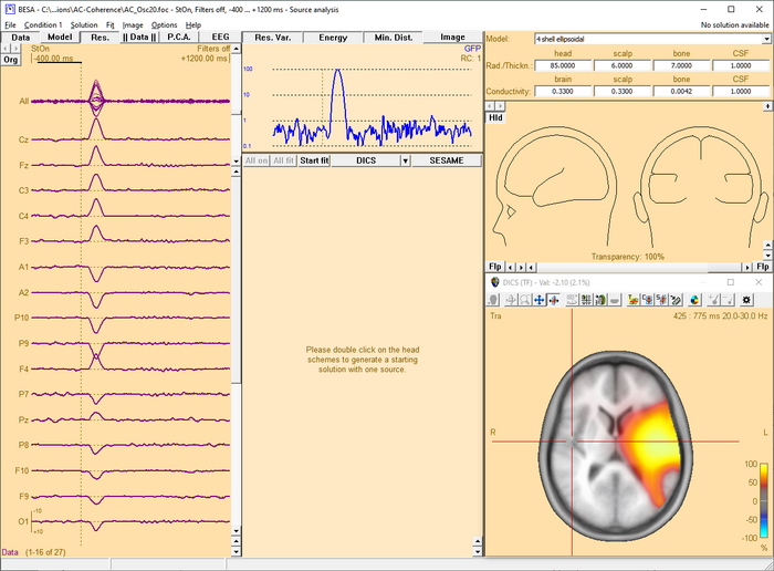
In case DICS is to be re-computed with a different reference, simply mark the desired reference position by placing the cross-hair in the anatomical view and select “DICS” in the middle panel of the source analysis window (see Fig. 4). In case an external reference is to be selected, click on “DICS” in the middle panel to bring up the DICS dialogue (see. Fig. 2) and select the desired channel. Please note that DICS computation will only be available after running time-frequency analysis. | In case DICS is to be re-computed with a different reference, simply mark the desired reference position by placing the cross-hair in the anatomical view and select “DICS” in the middle panel of the source analysis window (see Fig. 4). In case an external reference is to be selected, click on “DICS” in the middle panel to bring up the DICS dialogue (see. Fig. 2) and select the desired channel. Please note that DICS computation will only be available after running time-frequency analysis. | ||
| − | [[Image:SA 3Dimaging (23). | + | [[Image:SA 3Dimaging (23).png|700px|thumb|c|none|Fig. 4: Integration of DICS in the Source Analysis window]] |
== Multiple Source Beamformer (MSBF) in the Time Domain == | == Multiple Source Beamformer (MSBF) in the Time Domain == | ||
| − | '' | + | ''This feature requires BESA Research 7.0 or higher.'' |
| − | + | '''Short mathematical introduction''' | |
| + | |||
| + | Beamforming approach can be also applied in the time domain data. This approach was introduced as linearly constrained minimum variance (LCMV) beamformer (Van Veen et al., 1997). It allows to image evoked activity in a user-defined time range, where time is taken relative to a triggered event, and to estimate source waveforms using the calculated spatial weight at locations of interest. For an implementation of the beamformer in the time domain, data covariance matrices are required, while complex cross spectral density matrices are used for the beamformer approaches in the time-frequency domain as described in the ''[[Source_Analysis_3D_Imaging#Multiple_Source_Beamformer_.28MSBF.29_in_the_Time-frequency_Domain|Multiple Source Beamformer (MSBF) in the Time-frequency Domain]]'' section. | ||
| − | + | The bilateral beamformer introduced in the ''[[Source_Analysis_3D_Imaging#Multiple_Source_Beamformer_.28MSBF.29_in_the_Time-frequency_Domain|Multiple Source Beamformer (MSBF) in the Time-frequency Domain]]'' section is also implemented for the time-domain beamformer to take into account contributions from the homologue source in the opposite. This allows for imaging of highly correlated bilateral activity in the two hemispheres that commonly occurs during processing of external stimuli. In addition, the beamformer computation can take into account possibly correlated sources at arbitrary locations. | |
| − | |||
The beamformer spatial weight W(r) for the voxel r in the brain is defined as follows (Van Veen et al., 1997): | The beamformer spatial weight W(r) for the voxel r in the brain is defined as follows (Van Veen et al., 1997): | ||
| − | |||
| − | + | <math>\mathrm{W}(r) = [\mathrm{L}^T(r)\mathrm{C}^{-1}\mathrm{L}(r)]^{-1}\mathrm{L}^T(r)\mathrm{C}^{-1}</math> | |
| − | + | <!-- [[File:MSBF1.png]] --> | |
| − | + | ||
| − | |||
| − | where '''S'''(r,t) represents the estimated source waveform and '''M'''(t) represents measured EEG or MEG signals. | + | where <math>\mathrm{C}^{-1}</math> is the inversed regularized average of covariance matrix over trials, '''L''' is the leadfield matrix of the model containing a regional source at target location r and optionally additional sources whose interference with the target source is to be minimized. The beamformer spatial weight '''W'''(r) can be applied to the measured data to estimate source waveform at a location r (beamformer virtual sensor): |
| − | The output power P of the beamformer for a specific brain region at location r is computed by the following equation: | + | |
| + | |||
| + | <math>\mathrm{S}(r,t) = \mathrm{W}(r)\mathrm{M}(t)</math> | ||
| + | <!-- [[File:MSBF2.png]] --> | ||
| + | |||
| + | |||
| + | where '''S'''(r,t) represents the estimated source waveform and '''M'''(t) represents measured EEG or MEG signals. The output power P of the beamformer for a specific brain region at location r is computed by the following equation: | ||
| + | |||
| + | |||
| + | <math>\mathrm{P}(r) = \operatorname{tr^{'}}[\mathrm{W}(r) \cdot \mathrm{C} \cdot \mathrm{W}^T(r)]</math> | ||
| + | <!-- [[File:MSBF3.png]] --> | ||
| − | |||
where tr’[ ] is the trace of the [3×3] (MEG: [2×2]) submatrix of the bracketed expression that corresponds to the source at target location r. | where tr’[ ] is the trace of the [3×3] (MEG: [2×2]) submatrix of the bracketed expression that corresponds to the source at target location r. | ||
| − | |||
| − | |||
| − | |||
| − | |||
| − | |||
| − | + | Beamformer can suppress noise sources that are correlated across sensors. However, uncorrelated noise will be amplified in a spatially non-uniform manner, with increasing distortion with increasing distance from the sensors (Van Veen et al., 1997; Sekihara et al., 2001). For this reason, estimated source power should be normalized by a noise power. In BESA Research, the output power P(r) is normalized with the output power in a baseline interval or with the output power of a uncorrelated noise: P(r) / Pref (r). | |
| − | + | The time-domain beamformer image is constructed from values q(r) computed for all locations on a grid specified in the '''<u>General Settings</u>''' tab. A value q(r) is defined as described in | |
| + | the ''[[Source_Analysis_3D_Imaging#Multiple_Source_Beamformer_.28MSBF.29_in_the_Time-frequency_Domain|Multiple Source Beamformer (MSBF) in the Time-frequency Domain]]'' section with data covariance matrices instead of cross-spectral density matrices. | ||
| − | ''' | + | '''Applying the Beamformer''' |
| − | + | This chapter illustrates the usage of the BESA beamformer in the time domain. The displayed figures are generated using the file ‘Examples/ERP-Auditory-Intensity/S1.cnt’. | |
| − | + | ||
| − | + | ||
| − | + | '''''Starting the time-domain beamformer from the Average tab of the Paradigm dialog box''''' | |
| − | + | The time-domain beamformer is needed data covariance matrices and therefore requires the ERP module to be enabled. After the beamformer computation has been initiated in the '''<u>Average tab of the Paradigm dialog box</u>''', the source analysis window opens with an enlarged 3D image of the q-value computed with a bilateral beamformer. The result is superimposed onto the MR image assigned to the data set (individual or standard). | |
| − | + | ||
| + | [[File:MSBF4.png|500px|thumb|c|none|Beamformer image for auditory evoked data after starting the computation in the '''<u>Average tab of the Paradigm dialog box'''</u>. The bilateral beamformer manages to separate the activities in auditory areas, while a traditional single-source beamformer would merge the two sources into one image maximum in the head center instead.]] | ||
| − | '''Multiple-source beamformer in the Source Analysis window''' | + | '''''Multiple-source beamformer in the Source Analysis window''''' |
| − | The 3D imaging display is part of the source analysis window. In the Channel box, the averaged (evoked) data of the selected condition is shown. Selected covariance intervals in | + | The 3D imaging display is part of the source analysis window. In the Channel box, the averaged (evoked) data of the selected condition is shown. Selected covariance intervals in the ERP module can be checked in the Channel box. The red, gray, and blue rectangles indicate signal, baseline, and common interval, respectively. |
| − | the ERP module can be checked in the Channel box. The red, gray, and blue rectangles indicate signal, baseline, and common interval, respectively. | + | |
| − | [[File:MSBF55.png]] | + | [[File:MSBF55.png|700px|thumb|c|none|Source Analysis window with beamformer image. The two beamformer virtual sensors have been added using the Switch to Maximum and Add Source toolbar buttons (see below). |
| + | Source waveforms are computed using the beamformer spatial weights and the displayed averaged data (the noise normalized weights (5% noise) option was used to compute the beamformer image).]] | ||
| − | |||
| − | |||
| − | |||
When starting the beamformer from the '''<u>Average tab of the Paradigm dialog box</u>''', the bilateral beamformer scan is performed. In the source analysis window, the beamformer computation can be repeated taking into account possibly correlated sources that are specified in the current solution. Interfering activities generated by all sources in the current solution that are in the 'On' state are specifically suppressed (they enter the leadfield matrix L in the beamformer calculation). The computation can be started from the '''<u>Image</u>''' menu or from the Image selector button [[File:MSBF_Button.png|22px|Image: 22 pixels]] dropdown menu. The Image menu can be evoked either from the menu bar or by right-clicking anywhere in the source analysis window. | When starting the beamformer from the '''<u>Average tab of the Paradigm dialog box</u>''', the bilateral beamformer scan is performed. In the source analysis window, the beamformer computation can be repeated taking into account possibly correlated sources that are specified in the current solution. Interfering activities generated by all sources in the current solution that are in the 'On' state are specifically suppressed (they enter the leadfield matrix L in the beamformer calculation). The computation can be started from the '''<u>Image</u>''' menu or from the Image selector button [[File:MSBF_Button.png|22px|Image: 22 pixels]] dropdown menu. The Image menu can be evoked either from the menu bar or by right-clicking anywhere in the source analysis window. | ||
| + | [[File:MSBF66.png|700px|thumb|c|none|Multiple-source beamformer image calculated in the presence of a source in the left hemisphere. A single-source scan has been performed instead of a bilateral beamforemr. The source set in the current solution accounts for the left-hemispheric q-maximum in the data. Accordingly, the beamformer scan reveals only the as yet unmodeled additional activity in the right hemisphere (note the radiological convention in the 3D image display). The source waveform of the beamformer virtual sensor in the left hemisphere is not shown since the location (blue square in the figure) is not considered for the multiple-source beamformer.]] | ||
| − | |||
| − | + | The beamformer scan can be performed with a single or a bilateral source scan. The default scan type depends on the current solution: | |
| − | + | ||
| − | + | ||
| − | + | ||
| + | When the beamformer is started from the '''<u>Average tab of the Paradigm dialog box</u>''' the Source Analysis window opens with a new solution and a bilateral beamformer scan is performed. | ||
| − | |||
| − | |||
| − | |||
When the beamformer is started within the Source Analysis window, the default is: | When the beamformer is started within the Source Analysis window, the default is: | ||
| − | |||
* a scan with a single source in addition to the sources in the current solution, if at least one source is active. | * a scan with a single source in addition to the sources in the current solution, if at least one source is active. | ||
* a bilateral scan if no source in the current solution is active. | * a bilateral scan if no source in the current solution is active. | ||
| Line 354: | Line 337: | ||
menu or in the beamformer option dialog box (only for the time-domain beamformer). | menu or in the beamformer option dialog box (only for the time-domain beamformer). | ||
| − | + | ||
| + | '''Inserting Sources as Beamformer Virtual Sensor out of the Beamformer Image''' | ||
This is similar to the inserting sources out of the beamformer image in Multiple Source Beamformer (MSBF) in the Time-frequency Domain section. | This is similar to the inserting sources out of the beamformer image in Multiple Source Beamformer (MSBF) in the Time-frequency Domain section. | ||
| − | The beamformer image can be used to add beamformer virtual sensors to the current solution. A simple double-click anywhere in the 3D view (not in the 2D view) will generate a | + | |
| − | source at the corresponding location. A better and easier way to create sources at image maxima and minima is to use the toolbar buttons ''' | + | The beamformer image can be used to add beamformer virtual sensors to the current solution. A simple double-click anywhere in the 3D view (not in the 2D view) will generate a source at the corresponding location. A better and easier way to create sources at image maxima and minima is to use the toolbar buttons <span style="color:#3366ff;">'''Switch to Maximum'''</span> [[Image:SA 3Dimaging (8).gif]] and <span style="color:#3366ff;">'''Add Source'''</span> [[Image:SA 3Dimaging (9).gif]]. |
This feature allows to use the beamformer as a tool to create a source montage for '''<u>source coherence</u>''' analysis. A source montage file (*.mtg) for beamformer virtual sensors can | This feature allows to use the beamformer as a tool to create a source montage for '''<u>source coherence</u>''' analysis. A source montage file (*.mtg) for beamformer virtual sensors can | ||
be saved using File \ Save Source Montage As… entry. | be saved using File \ Save Source Montage As… entry. | ||
| − | The time-domain beamformer image can be also used to add regional or dipole sources to the current solution. Press '''N''' key when there is no source in the current source array or | + | The time-domain beamformer image can be also used to add regional or dipole sources to the current solution. Press '''N''' key when there is no source in the current source array or there is more than one beamformer virtual sensor. To create a new source array for beamformer virtual sensor, press '''N''' key when there is more than one regional or dipole source in the current source array. |
| − | there is more than one beamformer virtual sensor. To create a new source array for beamformer virtual sensor, press '''N''' key when there is more than one regional or dipole source in | + | |
| − | the current source array. | + | |
| − | + | '''Notes''' | |
* You can hide or re-display the last computed image by selecting ''Hide Image'' entry in the '''<u>Image</u>''' menu. | * You can hide or re-display the last computed image by selecting ''Hide Image'' entry in the '''<u>Image</u>''' menu. | ||
| − | * The current image can be exported to ASCII, ANALYZE, or BrainVoyager (vmp) format from the '''<u>Image</u>''' menu. | + | * The current image can be exported to ASCII, ANALYZE, or BrainVoyager (*.vmp) format from the '''<u>Image</u>''' menu. |
| − | * For scaling options, use | + | * For scaling options, use [[Image:SA 3Dimaging (10).gif]] and [[Image:SA 3Dimaging (11).gif]] <span style="color:#3366ff;">'''Image Scale toolbar'''</span> buttons. |
* Parameters used for the beamformer calculations can be set in the '''Standard Volume tab of the Image Settings <u>dialog box</u>'''. | * Parameters used for the beamformer calculations can be set in the '''Standard Volume tab of the Image Settings <u>dialog box</u>'''. | ||
* Note that Model, Residual, Order, and Residual variance are not shown for the beamformer virtual sensor type sources. | * Note that Model, Residual, Order, and Residual variance are not shown for the beamformer virtual sensor type sources. | ||
| − | + | ||
| + | '''References''' | ||
* Sekihara, K., Nagarajan, S. S., Poeppel, D., Marantz, A., & Miyashita, Y. (2001). Reconstructing spatio-temporal activities of neural sources using an MEG vector beamformer technique. IEEE Transactions on Biomedical Engineering, 48(7), 760–771. | * Sekihara, K., Nagarajan, S. S., Poeppel, D., Marantz, A., & Miyashita, Y. (2001). Reconstructing spatio-temporal activities of neural sources using an MEG vector beamformer technique. IEEE Transactions on Biomedical Engineering, 48(7), 760–771. | ||
| Line 427: | Line 411: | ||
| − | + | where | |
| Line 551: | Line 535: | ||
| − | The sLORETA image in BESA Research displays the norm of S<sub>sLORETA</sub>, r at each location r. Using the menu function ''Image / Export Image As...'' you have the option to save this norm of S<sub>sLORETA</sub>, <sub>r</sub> or alternatively all components separately to disk. | + | The sLORETA image in BESA Research displays the norm of S<sub>sLORETA</sub>, <sub>r</sub> at each location r. Using the menu function ''Image / Export Image As...'' you have the option to save this norm of S<sub>sLORETA</sub>, <sub>r</sub> or alternatively all components separately to disk. |
| Line 557: | Line 541: | ||
* sLORETA can be started from the <span style="color:#3366ff;">'''Image'''</span> menu or from the <span style="color:#3366ff;">'''Image Selection'''</span> button. | * sLORETA can be started from the <span style="color:#3366ff;">'''Image'''</span> menu or from the <span style="color:#3366ff;">'''Image Selection'''</span> button. | ||
| − | * Please refer to Chapter | + | * Please refer to Chapter [[#Regularization_of_distributed_volume_images|''Regularization of distributed volume images'']] for important information on regularization of distributed inverses. |
== swLORETA == | == swLORETA == | ||
| Line 588: | Line 572: | ||
| − | The swLORETA image in BESA Research displays the norm of S<sub>swLORETA</sub>, r at each location r. Using the menu function ''Image / Export Image As...'' you have the option to save this norm of S<sub>swLORETA</sub>, r or alternatively all components separately to disk. | + | The swLORETA image in BESA Research displays the norm of S<sub>swLORETA</sub>, <sub>r</sub> at each location r. Using the menu function ''Image / Export Image As...'' you have the option to save this norm of S<sub>swLORETA</sub>, <sub>r</sub> or alternatively all components separately to disk. |
| Line 628: | Line 612: | ||
| − | Here, L is the leadfield matrix of the distributed source model with regional sources distributed on a regular cubic grid. D(t) is the data at time point t. Custom-defined parameters are: | + | Here, L is the leadfield matrix of the distributed source model with regional sources distributed on a regular cubic grid. D(t) is the data at time point t. Custom-defined parameters are: |
| − | * Regularization: The term in parentheses is generally regularized. Note that regularization has a strong effect on the obtained results. Please refer to chapter | + | * '''The spatial weighting matrix V''': This may include depth weighting, image weighting, or cross-voxel weighting with a 3D Laplacian (as in LORETA) or an autoregressive function (as in LAURA). |
| − | * Standardization: Optionally, the result of the distributed inverse can be standardized with the resolution matrix (as in sLORETA). | + | * '''Regularization''': The term in parentheses is generally regularized. Note that regularization has a strong effect on the obtained results. Please refer to chapter ''Regularization of Distributed Volume Images''for more information. |
| − | * Iterations: Inverse computations can be applied iteratively. Each iteration is weighted with the image obtained in the previous iteration. | + | * '''Standardization''': Optionally, the result of the distributed inverse can be standardized with the resolution matrix (as in sLORETA). |
| + | * '''Iterations''': Inverse computations can be applied iteratively. Each iteration is weighted with the image obtained in the previous iteration. | ||
| − | All parameters for the user-defined volume image are specified in the User-Defined Volume Tab of the Image Settings dialog box. Please refer to chapter | + | All parameters for the user-defined volume image are specified in the User-Defined Volume Tab of the Image Settings dialog box. Please refer to chapter ''User-Defined Volume Tab'' for details. |
'''Notes:''' | '''Notes:''' | ||
| + | |||
* Starting the user-defined volume image: the image calculation can be started from the <span style="color:#3366ff;">'''Image'''</span> menu or from the <span style="color:#3366ff;">'''Image Selection'''</span> button. | * Starting the user-defined volume image: the image calculation can be started from the <span style="color:#3366ff;">'''Image'''</span> menu or from the <span style="color:#3366ff;">'''Image Selection'''</span> button. | ||
| − | * Please refer to Chapter | + | * Please refer to Chapter ''Regularization of distributed volume images'' for important information on regularization of distributed inverses. |
== Regularization of distributed volume images == | == Regularization of distributed volume images == | ||
| Line 646: | Line 632: | ||
* '''Tikhonov regularization''': In Tikhonov regularization, the term L V L<sup>T</sup> is inverted as (L V L<sup>T </sup>+λ I)<sup>-1</sup>. Here, l is the regularization constant, and I is the identity matrix. | * '''Tikhonov regularization''': In Tikhonov regularization, the term L V L<sup>T</sup> is inverted as (L V L<sup>T </sup>+λ I)<sup>-1</sup>. Here, l is the regularization constant, and I is the identity matrix. | ||
| − | * One way of determining the optimum regularization constant is by minimizing the ''generalized cross'' ''validation error'' (CVE). | + | ** One way of determining the optimum regularization constant is by minimizing the ''generalized cross'' ''validation error'' (CVE). |
| − | * Alternatively, the regularization constant can be specified manually as a percentage of the trace of the matrix L V L<sup>T</sup>. | + | ** Alternatively, the regularization constant can be specified manually as a percentage of the trace of the matrix L V L<sup>T</sup>. |
* '''TSVD''': In the truncated singular value decomposition (TSVD) approach, an SVD decomposition of L V L<sup>T</sup> is computed as L V L<sup>T</sup> = U S U<sup>T</sup>, where the diagonal matrix S contains the singular values. All singular values smaller than the specified percentage of the maximum singular values are set to zero. The inverse is computed as U S<sup>-1</sup> U<sup>T</sup>, where the diagonal elements of S<sup>-1 </sup>are the inverse of the corresponding non-zero diagonal elements of S. | * '''TSVD''': In the truncated singular value decomposition (TSVD) approach, an SVD decomposition of L V L<sup>T</sup> is computed as L V L<sup>T</sup> = U S U<sup>T</sup>, where the diagonal matrix S contains the singular values. All singular values smaller than the specified percentage of the maximum singular values are set to zero. The inverse is computed as U S<sup>-1</sup> U<sup>T</sup>, where the diagonal elements of S<sup>-1 </sup>are the inverse of the corresponding non-zero diagonal elements of S. | ||
| Line 653: | Line 639: | ||
Regularization has a critical effect on the obtained distributed source images. The results may differ completely with different choices of the regularization parameter (see examples below). Therefore, it is important to evaluate the generated image critically with respect to the regularization constant, and to keep in mind the uncertainties resulting from this fact when interpreting the results. The default setting in BESA Research is a TSVD regularization with a 0.03% threshold. However, this value might need to be adjusted to the specific data set at hand. | Regularization has a critical effect on the obtained distributed source images. The results may differ completely with different choices of the regularization parameter (see examples below). Therefore, it is important to evaluate the generated image critically with respect to the regularization constant, and to keep in mind the uncertainties resulting from this fact when interpreting the results. The default setting in BESA Research is a TSVD regularization with a 0.03% threshold. However, this value might need to be adjusted to the specific data set at hand. | ||
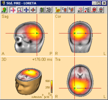
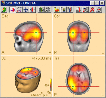
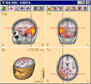
| − | The following example illustrates the influence of the regularization parameter on the obtained images. The data used here is condition <span style="color:#ff9c00;">'''St-Cor of dataset Examples \ TFC-Error-Related-Negativity \ Correct+Error.fsg'''</span> at 176 ms following the visual stimulus. Discrete dipole analysis reveals the main activity in the left and right lateral visual cortex at this latency. | + | The following example illustrates the influence of the regularization parameter on the obtained images. The data used here is condition <span style="color:#ff9c00;">'''St-Cor </span> of dataset <span style="color:#ff9c00;">Examples \ TFC-Error-Related-Negativity \ Correct+Error.fsg'''</span> at 176 ms following the visual stimulus. Discrete dipole analysis reveals the main activity in the left and right lateral visual cortex at this latency. |
| − | + | ||
| − | + | ||
| − | + | ||
| − | + | [[File:SA 3Dimaging (42).gif|400px|thumb|c|none|Discrete source model at 176 ms: Main activity in the left and right lateral visual cortex, no visual midline activity.]] | |
| Line 664: | Line 647: | ||
<div><ul> | <div><ul> | ||
| − | <li style="display: inline-block;"> [[File:SA 3Dimaging ( | + | <li style="display: inline-block;"> [[File:SA 3Dimaging (44).gif|thumb|350px|'''SVD cutoff 0.1%''': Regularization too strong. No separation between sources, mislocalization towards the middle of the brain.]] </li> |
| − | <li style="display: inline-block;"> [[File:SA 3Dimaging ( | + | <li style="display: inline-block;"> [[File:SA 3Dimaging (43).gif|thumb|350px|'''SVD cutoff 0.005%''': Appropriate regularization. Separation of the bilateral activities. Location in agreement with the discrete multiple source model.]] </li> |
<li style="display: inline-block;"> [[File:SA 3Dimaging (45).gif|thumb|350px|'''SVD cutoff 0.0001%''':<br /> Too small regularization. Mislocalization, too superficial 3D image. ]] </li> | <li style="display: inline-block;"> [[File:SA 3Dimaging (45).gif|thumb|350px|'''SVD cutoff 0.0001%''':<br /> Too small regularization. Mislocalization, too superficial 3D image. ]] </li> | ||
</ul></div> | </ul></div> | ||
| − | |||
The automatic determination of the regularization constant using the CVE approach does not necessarily result in the optimum regularization parameter either. In this example, the unscaled CVE approach rather resembles the TSVD image with a cutoff of 0.0001%, i.e. regularization is too small. Therefore, it is advisable to compare different settings of the regularization parameter and make the final choice based on the above-mentioned considerations. | The automatic determination of the regularization constant using the CVE approach does not necessarily result in the optimum regularization parameter either. In this example, the unscaled CVE approach rather resembles the TSVD image with a cutoff of 0.0001%, i.e. regularization is too small. Therefore, it is advisable to compare different settings of the regularization parameter and make the final choice based on the above-mentioned considerations. | ||
| Line 739: | Line 721: | ||
'''Regularization and other parameters:''' | '''Regularization and other parameters:''' | ||
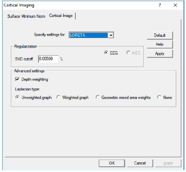
| − | [[Image: | + | [[Image:CorticalLOR.png]] |
* '''SVD cutoff''': The regularization for the inverse operator as a percent of the largest singular value. | * '''SVD cutoff''': The regularization for the inverse operator as a percent of the largest singular value. | ||
| Line 749: | Line 731: | ||
* '''Starting Cortical LORETA''': Cortical LORETA can be started from the sub-menu <span style="color:#3366ff;">'''Surface </span><span style="color:#3366ff;">Image'''</span> of the <span style="color:#3366ff;">'''Image'''</span> menu or from the <span style="color:#3366ff;">'''Image Selection'''</span> button. | * '''Starting Cortical LORETA''': Cortical LORETA can be started from the sub-menu <span style="color:#3366ff;">'''Surface </span><span style="color:#3366ff;">Image'''</span> of the <span style="color:#3366ff;">'''Image'''</span> menu or from the <span style="color:#3366ff;">'''Image Selection'''</span> button. | ||
* Please refer to Chapter “''[[Source_Analysis_3D_Imaging#Regularization_of_distributed_volume_images|Regularization of distributed volume images]]''” for important information on regularization of distributed inverses. | * Please refer to Chapter “''[[Source_Analysis_3D_Imaging#Regularization_of_distributed_volume_images|Regularization of distributed volume images]]''” for important information on regularization of distributed inverses. | ||
| + | |||
| + | |||
| + | '''References:''' | ||
| + | |||
| + | Please refer to ''Iordanov et al.: LORETA With Cortical Constraint: Choosing an Adequate Surface Laplacian Operator. Front Neurosci 12, Article 746, 2018'', for more information - full article available [https://www.frontiersin.org/articles/10.3389/fnins.2018.00746/full here]. | ||
== Cortical CLARA == | == Cortical CLARA == | ||
| Line 817: | Line 804: | ||
'''Noise regularization''' | '''Noise regularization''' | ||
| − | + | Three methods to estimate the channel noise correlation matrix C<sub>N</sub> are provided by the program: | |
* '''Use baseline:''' Select this option to estimate the noise from the user-definable baseline. The signal is computed from the data at non-baseline latencies. | * '''Use baseline:''' Select this option to estimate the noise from the user-definable baseline. The signal is computed from the data at non-baseline latencies. | ||
* '''Use 15% lowest values:''' The baseline activity is computed from the data at those 15% of all displayed latencies that have the lowest global field power. The signal is computed from all displayed latencies. | * '''Use 15% lowest values:''' The baseline activity is computed from the data at those 15% of all displayed latencies that have the lowest global field power. The signal is computed from all displayed latencies. | ||
| + | * '''Use the full baseline covariance matrix''': This option is only available if a previous beamformer image in the time-domain was calculated. In this case, it can be selected from the general image settings dialog tab. The baseline covariance interval is the one selected for the beamformer, and is indicated by a thin horizontal bar in the channel box. | ||
In each case, the activity (noise or signal, respectively) is defined as root-mean-square across all respective latencies for each channel. | In each case, the activity (noise or signal, respectively) is defined as root-mean-square across all respective latencies for each channel. | ||
| Line 899: | Line 887: | ||
<div><ul> | <div><ul> | ||
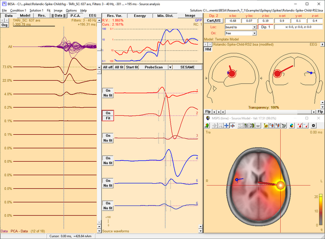
| − | <li style="display: inline-block;"> [[ | + | <li style="display: inline-block;"> [[File:SA 3Dimaging (55).png|thumb|c|none|650px|This figure shows the MSPS image applied on the three left-hemispheric sources in the solution '<span style="color:#ff9c00;">'''Rolandic-Spike-Child-RS2.bsa'''</span>'. The baseline is set from -300 ms to -50 ms. The right-hemispheric sources have been switched off. The fit interval is set to the latency range of large overall activity in the data (-43 ms : 117 ms). A realistic FEM model appropriate for the subject's age (12 years, conductivity ratios (cr) 50) is applied. The MSPS image does not show maxima at the modeled source locations and rather shows a spread q-value distribution.]] </li> |
| − | <li style="display: inline-block;"> [[ | + | <li style="display: inline-block;"> [[File:SA 3Dimaging (56).png|thumb|c|none|650px|The MSPS image for the same latency range when the right-hemispheric sources have been included. The MSPS image appears more focal and shows maxima around the modeled brain regions. This indicates the substantial improvement of the solution by adding the right-hemispheric sources that model the propagation of the epileptic spike from the left to the right hemisphere (note the radiological side convention in the 3D window).]] </li> |
</ul></div> | </ul></div> | ||
| Line 910: | Line 898: | ||
Time-resolved MSPS images are not available if the MSPS has been computed on data in the time-frequency domain. | Time-resolved MSPS images are not available if the MSPS has been computed on data in the time-frequency domain. | ||
| + | |||
<div><ul> | <div><ul> | ||
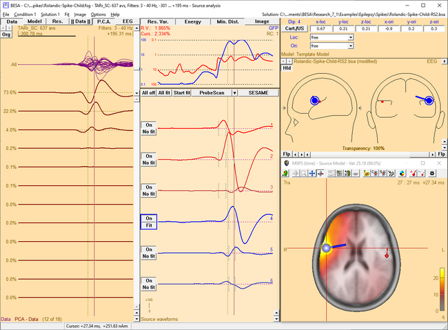
| − | <li style="display: inline-block;"> [[File:SA 3Dimaging (57). | + | <li style="display: inline-block;"> [[File:SA 3Dimaging (57).png|thumb|c|none|650px|MSPS image of the spike peak activity at 0 ms. The activity mainly occurs in the left hemisphere. This fact is illustrated by the source waveforms and confirmed in the MSPS image, which shows a focal maximum around the location of the red sources.]] </li> |
| − | <li style="display: inline-block;"> [[File:SA 3Dimaging (58). | + | <li style="display: inline-block;"> [[File:SA 3Dimaging (58).png|thumb|c|none|650px|Around +27 ms, the spike has propagated to the right hemisphere. This becomes evident from the waveforms of the blue sources, which show a significant latency lag with respect to the first three sources, and from the MSPS image, which shows the maximum around blue sources at this latency.]] </li> |
</ul></div> | </ul></div> | ||
| − | |||
| − | |||
| − | |||
| − | |||
| − | |||
| − | |||
| − | |||
| − | |||
| − | |||
| − | |||
| − | |||
| Line 961: | Line 939: | ||
| − | [[Image:SA 3Dimaging (59). | + | [[Image:SA 3Dimaging (59).png|700px|thumb|c|none|Source Sensitivity image for the selected frontal source (green) in model ''<span style="color:#ff9c00;">''''High_Intensity_3RS.bsa''''</span>'' in folder 'Examples/ERP_Auditory_Intensity'. The data displayed is the '100dB' condition in file ''<span style="color:#ff9c00;">''''All_Subjects_cc.fsg''''</span>''. The selected source is sensitive to activity in the frontal brain region (yellow/white), while it is not influenced by activity in the vicinity of the left and right auditory cortex areas, which are modeled by the red and blue source in the model (transparent/gray).]] |
| − | + | ||
| − | + | ||
| Line 972: | Line 948: | ||
* You can hide or re-display the last computed image by selecting the corresponding entry in the <span style="color:#3366ff;">'''Image'''</span> menu. | * You can hide or re-display the last computed image by selecting the corresponding entry in the <span style="color:#3366ff;">'''Image'''</span> menu. | ||
* The current image can be exported to ASCII or BrainVoyager vmp-format from the <span style="color:#3366ff;">'''Image'''</span> menu. | * The current image can be exported to ASCII or BrainVoyager vmp-format from the <span style="color:#3366ff;">'''Image'''</span> menu. | ||
| + | |||
| + | == SESAME == | ||
| + | |||
| + | ''This feature requires BESA Research 7.0 or higher.'' | ||
| + | |||
| + | '''SESAME''' (Sequential Semi-Analytic Monte-Carlo Estimation) is a Bayesian approach for estimating sources that uses Markov-Chain Monte-Carlo method for efficient computation of the probability distribution as described in Sommariva, S., & Sorrentino, A. "Sequential Monte Carlo samplers for semi-linear inverse problems and application to magnetoencephalography." Inverse Problems 30.11 (2014): 114020. | ||
| + | |||
| + | It allows to automatically estimate simultaneously the number of dipoles, their locations and time courses requiring virtually no user input. The algorithm is divided in two blocks: | ||
| + | |||
| + | * The first block consists of a Monte Carlo sampling algorithm that produces, with an adaptive number of iterations, a set of samples representing the posterior distribution for the number of dipoles and the dipole locations. | ||
| + | * The second block estimates the source time courses, given the number of dipoles and the dipole locations. | ||
| + | |||
| + | The Monte Carlo algorithm in the first block works by letting a set of weighted samples evolve with each iteration. At each iteration, the samples (a multi-dipole state) approximates the n-th element of a sequence of distributions p1, …, pN, that reaches the desired posterior distribution (pN = p(x|y)). The sequence is built as pN = p(x) p(y|x) α(n), such that α(1) = 0, α(N) = 1. The actual sequence of values of alpha is determined online. Dipole moments are estimated after the number of dipoles and the dipole locations have been estimated with the Monte Carlo procedure. This continues until a steady state is reached. | ||
| + | |||
| + | The SESAME image in BESA Research displays the final probability of source location along with an estimate for number of sources. Using the menu function <span style="color:#3366ff;">'''Image / Export Image As...'''</span> you have the option to save this SESAME image. | ||
| + | |||
| + | |||
| + | '''Non-uniform spatial priors for SESAME''' | ||
| + | |||
| + | By default, SESAME uses a uniform prior distribution on the source location. However, when the Weight by Image button at the top of the variance box is pressed and SESAME image is computed, the currently active 3D image will be used as non-uniform spatial priors for the SESAME computation (the positive values in the active 3D image, scaled to the current image maximum, are used as non-uniform spatial priors). The usage of non-uniform priors can effectively increase the source localization accuracy when the prior distribution is correct (A. Viani, G. Luria and A. Sorrentino, "Non-uniform spatial priors for multi-dipole localization from MEG/EEG data," 2022 IEEE International Conference on E-health Networking, Application & Services (HealthCom), Genoa, Italy, 2022, pp. 149-154, doi: 10.1109/HealthCom54947.2022.9982792). | ||
| + | To use this method, a 3D image (e.g. source image or imported fMRI image) should be displayed in the 3D window. | ||
| + | When the computation is finished, the Weight by Image button will be released. | ||
| + | |||
| + | |||
| + | '''Notes:''' | ||
| + | |||
| + | *'''Grid spacing:''' Due to memory and computational limitations, it is recommended to use SESAME with a grid spacing of 5 mm or more. | ||
| + | *'''Fit Interval:''' SESAME requires a fit interval of more than 2 samples to start the computation. | ||
| + | *'''Computation time:''' Computation speed during SESAME calculation depends on the grid spacing (computation is faster with larger grid spacing) and number of channels. | ||
| + | |||
| + | == Brain Atlas == | ||
| + | ''This feature requires BESA Research 7.0 or higher.'' | ||
| + | |||
| + | '''Introduction''' | ||
| + | |||
| + | Brain atlas is a priori data that can be applied over any discrete or distributed source image displayed in the 3D window. It is a reference value that strongly depends on the selected brain atlas and should not be used as medical reference since individual brains may differ from the brain atlas. The display settings can be adjusted in 3D Window Tab. | ||
| + | |||
| + | [[Image:BrainAtlas1.png|600px]] | ||
| + | |||
| + | |||
| + | '''Brain Atlases''' | ||
| + | |||
| + | In BESA Research the atlases listed below are provided. '''BESA is not the author of the atlases; please cite the appropriate publications if you use any of the atlases in your publication.''' | ||
| + | |||
| + | [http://atlas.brainnetome.org/bnatlas.html '''Brainnetome'''] <br> | ||
| + | This is one of the most modern brain probabilistic atlas where structural, functional, and connectivity information was used to perform cortical parcellation. It was introduce by Fan and colleagues (2016), and is still work in progress. The atlas was created using data from 40 healthy adults taking part in the Human Connectome Project. In March 2018, the atlas consists of 246 structures labeled independently for each hemisphere. In BESA we provide the max probability map with labeling. Please visit the Brainnetome webpage to see more details related to the indicated brain regions (i.e. behavioral domains, paradigm classes and regions connectivity). | ||
| + | |||
| + | '''AAL''' <br> | ||
| + | Automated Anatomical Labeling atlas was created in 2002 by Tzourio-Mazoyer and collegues (2002). It is the mostly used atlas nowadays. The atlas is based on the averaged brain of one subject (young male) who was scanned 27 times. The atlas resolution is 1 mm isometric. The brain sulci were drawn manually on every 2mm slice and then brain regions were automatically assigned. The atlas consists of 116 regions which are asymmetrical between hemispheres. The atlas is implemented as in the [https://www.fil.ion.ucl.ac.uk/spm/ '''SPM12'''] toolbox. | ||
| + | |||
| + | '''Brodmann''' <br> | ||
| + | The Brodmann map was created by Brodmann (1909). The brain regions were differentiated by cytoarchitecture of each cortical area using the Nissi method of cell staining. The digitalization of the original Brodmann map was performed by Damasio and Damasio (1989). The digitalized atlas consists of 44 fields that are symmetric between hemispheres. BESA used the atlas implementation as in Chris Roden’s [https://people.cas.sc.edu/rorden/mricro/index.html '''MRICro'''] software. | ||
| + | |||
| + | '''AAL2015''' <br> | ||
| + | Automated Anatomical Labeling revision 2015. This is the updated AAL atlas. In comparison to the previous version (AAL) mainly the frontal lobe shows a higher degree of parcellation (Rolls, Joliot, and Tzourio-Mazoyer 2015). The atlas is implemented as in the [https://www.fil.ion.ucl.ac.uk/spm/ '''SPM12'''] toolbox. | ||
| + | |||
| + | '''Talairach''' <br> | ||
| + | Atlas was created in 1988 by Talairach and Tournoux (1988) and it is based on the post mortem brain slices of a 60 year old right handed European female. It was created by drawing and matching regions with the Brodmann map. The atlas is available at 5 tissue levels, however we used only the volumetric gyrus level as it is the most known in neuroscience and is the most appropriate for EEG. The atlas consists of 55 regions that are symmetric between hemispheres. The native resolution of the atlas was 0.43x0.43x2-5 mm. Please note that the poor resolution in Z direction is a direct consequence atlas definition, and since it is a post-mortem atlas it will not correctly match the brain template | ||
| + | (noticeable mainly on brain edges). The atlas digitalization was performed by Lancaster and colleagues (2000) resulting in a “golden standard” for neuroscience. The atlas was first implemented in a software called [http://www.talairach.org/daemon.html '''talairach daemon''']. | ||
| + | |||
| + | '''Yeo7 and Yeo17''' <br> | ||
| + | Yeo7 and Yeo17 are the resting state functional connectivity atlases created by Yeo et al. (2011). For atlas creation 1000 subjects, coregistered using surface-based alignment were used. Two versions of parcellation were used resulting for the 7 and 17 networks (Yeo7 and Yeo17 atlas respectively). In the original publication atlases for two different levels of brain structure coverage were prepared: neocortex and liberal. In BESA products, only one of them (liberal) is available. Note that in comparison to the other atlases, here networks are reflected, rather than the individual brain structures. These atlases are in line with [[BESA_Research_Montage_Editor#Standard_Source_Montage_-_Resting_State_Montages | Resting State Source Montages]]. | ||
| + | |||
| + | |||
| + | '''Visualization modes''' | ||
| + | |||
| + | '''Just Labels''' <br> | ||
| + | Displayed are crosshair coordinates (Talairach or MNI), the currently used brain atlas and the region name where the crosshair is placed. No atlas overlay will be visible on the 3D image. | ||
| + | |||
| + | '''brainCOLOR''' <br> | ||
| + | All information is displayed as in “Just Labels” mode but also the atlas is visible as an overlay over the MRI. The coloring is performed using the algorithm introduced by Klein and colleagues (Klein et al. 2010). With this method of coloring the regions which are part of the same lobe are colored in a similar color but with different color shade. The shade is computed by the algorithm to make these regions visually differentiable from each other as much as possible. | ||
| + | |||
| + | '''Individual Color''' <br> | ||
| + | In this mode the native brain atlas color is used if provided by the authors of the brain atlas (i.e. Yeo7). Where this was not available BESA autogenerated colors for the atlas using an approach similar to political map coloring. This approach aims to differentiate most regions that are adjacent to each other and no presumptions on lobes is applied. | ||
| + | |||
| + | '''Contour''' <br> | ||
| + | Only region contours (borders between atlas regions) are drawn with blue color. This is the default mode in BESA Research. | ||
| + | |||
| + | |||
| + | '''References''' | ||
| + | |||
| + | * Brodmann, Korbinian. 1909. Vergleichende Lokalisationslehre Der Großhirnrinde. Leipzig: Barth. https://www.livivo.de/doc/437605. | ||
| + | * Damasio, Hanna, and Antonio R. Damasio. 1989. Lesion Analysis in Neuropsychology. Oxford University Press, USA. | ||
| + | * Fan, Lingzhong, Hai Li, Junjie Zhuo, Yu Zhang, Jiaojian Wang, Liangfu Chen, Zhengyi Yang, et al. 2016. “The Human Brainnetome Atlas: A New Brain Atlas Based on Connectional Architecture.” Cerebral Cortex 26 (8): 3508–26. https://doi.org/10.1093/cercor/bhw157. | ||
| + | * Klein, Arno, Andrew Worth, Jason Tourville, Bennett Landman, Tito Dal Canton, Satrajit S. Ghosh, and David Shattuck. 2010. “An Interactive Tool for Constructing Optimal Brain Colormaps.” https://mindboggle.info/braincolor/colormaps/index.html. | ||
| + | * Lancaster, Jack L., Marty G. Woldorff, Lawrence M. Parsons, Mario Liotti, Catarina S. Freitas, Lacy Rainey, Peter V. Kochunov, Dan Nickerson, Shawn A. Mikiten, and Peter T. Fox. 2000. “Automated Talairach Atlas Labels for Functional Brain Mapping.” Human Brain Mapping 10 (3): 120–131. | ||
| + | *Rolls, Edmund T., Marc Joliot, and Nathalie Tzourio-Mazoyer. 2015. “Implementation of a New Parcellation of the Orbitofrontal Cortex in the Automated Anatomical Labeling Atlas.” NeuroImage 122 (November): 1–5. https://doi.org/10.1016/j.neuroimage.2015.07.075. | ||
| + | * Talairach, J, and P Tournoux. 1988. Co-Planar Stereotaxic Atlas of the Human Brain. 3-Dimensional Proportional System: An Approach to Cerebral Imaging. Thieme. | ||
| + | *Thomas Yeo, B. T., F. M. Krienen, J. Sepulcre, M. R. Sabuncu, D. Lashkari, M. Hollinshead, J. L. Roffman, et al. 2011. “The Organization of the Human Cerebral Cortex Estimated by Intrinsic Functional Connectivity.” Journal of Neurophysiology 106 (3): 1125–65. https://doi.org/10.1152/jn.00338.2011. | ||
| + | * Tzourio-Mazoyer, N., B. Landeau, D. Papathanassiou, F. Crivello, O. Etard, N. Delcroix, B. Mazoyer, and M. Joliot. 2002. “Automated Anatomical Labeling of Activations in SPM Using a Macroscopic Anatomical Parcellation of the MNI MRI Single-Subject Brain.” NeuroImage 15 (1): 273–89. https://doi.org/10.1006/nimg.2001.0978. | ||
| + | |||
| + | == Slice View == | ||
| + | |||
| + | ''This feature requires BESA Research 7.1 or higher.'' | ||
| + | |||
| + | A convenient way to review MRI data and export it in graphical form is a multi-slice view. To enable multi-slice view press the toggle multiple view button until the slice view is shown in the 3D window. | ||
| + | |||
| + | [[Image:SliceView1.png|600px]] | ||
| + | |||
| + | In this view discrete sources, [[Source_Analysis_3D_Imaging#Overview | distributed sources]] and [[Source_Analysis_3D_Imaging#Brain Atlas| brain atlas]] can be also be overlayed. The display matrix can be adjusted by slice view controls that are available in the 3D Window tab of the Preferences Dialog Box. One of the following slicing direction can be selected: Transverse, Coronal, Sagittal by pressing the appropriate button in the 3D window toolbar. | ||
| + | |||
| + | By adjusting First slice and Last slice sliders, the span of the volume that will be displayed can be adjusted. The interval between slices can be adjusted by changing the Spacing slider value. The layout of slices will be automatically adjusted to fill the full space of the main window. All values in the sliders are given in mm. | ||
| + | |||
| + | '''Note''': The last slice value will be adjusted to the closest possible number matching the given first slice and spacing value. During multi-slice view the cursor is disabled and no | ||
| + | atlas information is provided. | ||
| + | |||
| + | == Glassbrain == | ||
| + | |||
| + | ''This feature requires BESA Research 7.1 or higher.'' | ||
| + | |||
| + | [[Image:Glassbrain.png|600px]] | ||
| + | |||
| + | The glass brain can be enabled or disabled in one of the following ways: | ||
| + | |||
| + | * by pressing the button [[File:Buton GlassBrain.png]] in the toolbar, | ||
| + | * by using the shortcut SHIFT-G or | ||
| + | * by checking the checkbox in Preferences, 3D Display tab. | ||
| + | |||
| + | The transparency value of the glass brain can be adjusted in one of the following ways: | ||
| + | |||
| + | * by a slider/edit box in Preferences, 3D Display tab or | ||
| + | * by using the keyboard shortcut SHIFT-UP (to increase transparency by 10%) or SHIFT-DOWN (to decrease transparency by 10%). | ||
| + | |||
| + | Note that If a distributed solution is displayed together with the glass brain, a notification is displayed in the left bottom corner of 3D window to prevent misconception of the glass brain as a cortical image: | ||
| + | |||
| + | “Volume-based image only", which means that the results of distributed source analysis images are visualized only for the current MRI slice, and are not projected to the displayed surface. | ||
| + | |||
{{BESAManualNav}} | {{BESAManualNav}} | ||
Latest revision as of 14:21, 11 March 2024
| Module information | |
| Modules | BESA Research Standard or higher |
| Version | BESA Research 6.1 or higher |
Contents
- 1 Overview
- 2 Multiple Source Beamformer (MSBF) in the Time-frequency Domain
- 3 Dynamic Imaging of Coherent Sources (DICS)
- 4 Multiple Source Beamformer (MSBF) in the Time Domain
- 5 CLARA
- 6 LAURA
- 7 LORETA
- 8 sLORETA
- 9 swLORETA
- 10 sSLOFO
- 11 User-Defined Volume Image
- 12 Regularization of distributed volume images
- 13 Cortical LORETA
- 14 Cortical CLARA
- 15 Cortex Inflation
- 16 Surface Minimum Norm Image
- 17 Multiple Source Probe Scan (MSPS)
- 18 Source Sensitivity
- 19 SESAME
- 20 Brain Atlas
- 21 Slice View
- 22 Glassbrain
Overview
BESA Research features a set of new functions that provide 3D images that are displayed superimposed to the individual subject's anatomy. This chapter introduces these different images and describe their properties and applications.
The 3D images can be divided into three categories:
Volume images:
- The Multiple Source Beamformer (MSBF) is a tool for imaging brain activity. It is applied in the time-domain or time-frequency domain. The beamformer technique in time-frequency domain can image not only evoked, but also induced activity, which is not visible in time-domain averages of the data.
- Dynamic Imaging of Coherent Sources (DICS) can find coherence between any two pairs of voxels in the brain or between an external source and brain voxels. DICS requires time-frequency-transformed data and can find coherence for evoked and induced activity.
The following imaging methods provide an image of brain activity based on a distributed multiple source model:
- CLARA is an iterative application of LORETA images, focusing the obtained 3D image in each iteration step.
- LAURA uses a spatial weighting function that has the form of a local autoregressive function.
- LORETA has the 3D Laplacian operator implemented as spatial weighting prior.
- sLORETA is an unweighted minimum norm that is standardized by the resolution matrix.
- swLORETA is equivalent to sLORETA, except for an additional depth weighting.
- SSLOFO is an iterative application of standardized minimum norm images with consecutive shrinkage of the source space.
- A User-defined volume image allows to experiment with the different imaging techniques. It is possible to specify user-defined parameters for the family of distributed source images to create a new imaging technique.
- Bayesian source imaging: SESAME uses a semi-automated Bayesian approach to estimate the number of dipoles along with their parameters.
Surface image:
- The Surface Minimum Norm Image. If no individual MRI is available, the minimum norm image is displayed on a standard brain surface and computed for standard source locations. If available, an individual brain surface is used to construct the distributed source model and to image the brain activity.
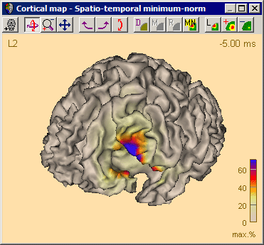
- Cortical LORETA. Unlike classical LORETA, cortical LORETA is not computed in a 3D volume, but on the cortical surface.
- Cortical CLARA. Unlike classical CLARA, cortical CLARA is not computed in a 3D volume, but on the cortical surface.
Discrete model probing:
These images do not visualize source activity. Rather, they visualize properties of the currently applied discrete source model:
- The Multiple Source Probe Scan (MSPS) is a tool for the validation of a discrete multiple source model.
- The Source Sensitivity image displays the sensitivity of a selected source in the current discrete source model and is therefore data independent.
Multiple Source Beamformer (MSBF) in the Time-frequency Domain
Short mathematical introduction
The BESA beamformer is a modified version of the linearly constrained minimum variance vector beamformer in the time-frequency domain as described in Gross et al., "Dynamic imaging of coherent sources: Studying neural interactions in the human brain", PNAS 98, 694-699, 2001. It allows to image evoked and induced oscillatory activity in a user-defined time-frequency range, where time is taken relative to a triggered event.
The computation is based on a transformation of each channel's single trial data from the time domain into the time-frequency domain. This transformation is performed by the BESA Research Source Coherence module and leads to the complex spectral density Si (f,t), where i is the channel index and f and t denote frequency and time, respectively. Complex cross spectral density matrices C are computed for each trial:
[math]\mathrm{C}_{ij}\left( f,t \right) = \mathrm{S}_{i}\left( f,t \right) \cdot \mathrm{S}_{j}^{*}\left( f,t \right)[/math]
The output power P of the beamformer for a specific brain region at location r is then computed by the following equation:
[math]\mathrm{P}\left( r \right) = \operatorname{tr^{'}}\left\lbrack \mathrm{L}^{T}\left( r \right) \cdot \mathrm{C}_{r}^{-1} \cdot \mathrm{L}\left( r \right) \right\rbrack^{-1}[/math]
Here, Cr-1 is the inverse of the SVD-regularized average of Cij(f,t) over trials and the time-frequency range of interest; L is the leadfield matrix of the model containing a regional source at target location r and, optionally, additional sources whose interference with the target source is to be minimized; tr'[] is the trace of the [3×3] (MEG:[2×2]) submatrix of the bracketed expression that corresponds to the source at target location r.
In BESA Research, the output power P(r) is normalized with the output power in a reference time-frequency interval Pref(r). A value q ist defined as follows:
[math] \mathrm{q}\left( r \right) =
\begin{cases}
\sqrt{\frac{\mathrm{P}\left( r \right)}{\mathrm{P}_{\text{ref}}(r)}} - 1 = \sqrt{\frac{\operatorname{tr^{'}}\left\lbrack \mathrm{L}^{T}\left( r \right) \cdot \mathrm{C}_{r}^{- 1} \cdot \mathrm{L}\left( r \right) \right\rbrack^{- 1}}{\operatorname{tr^{'}}\left\lbrack \mathrm{L}^{T}\left( r \right) \cdot \mathrm{C}_{\text{ref},r}^{- 1} \cdot \mathrm{L}\left( r \right) \right\rbrack^{- 1}}} - 1, & \text{for }\mathrm{P}(r) \geq \mathrm{P}_{\text{ref}}(r) \\
1 - \sqrt{\frac{\mathrm{P}_{\text{ref}}\left( r \right)}{\mathrm{P}\left( r \right)}} = 1 - \sqrt{\frac{\operatorname{tr^{'}}\left\lbrack \mathrm{L}^{T}\left( r \right) \cdot \mathrm{C}_{\text{ref},r}^{- 1} \cdot \mathrm{L}\left( r \right) \right\rbrack^{- 1}}{\operatorname{tr^{'}}\left\lbrack \mathrm{L}^{T}\left( r \right) \cdot \mathrm{C}_{r}^{- 1} \cdot \mathrm{L}\left( r \right) \right\rbrack^{- 1}}}, & \text{for }\mathrm{P}(r) \lt \mathrm{P}_{\text{ref}}(r)
\end{cases} [/math]
Pref can be computed either from the corresponding frequency range in the baseline of the same condition (i.e. the beamformer images event-related power increase or decrease) or from the corresponding time-frequency range in a control condition (i.e. the beamformer images differences between two conditions). The beamformer image is constructed from values q(r) computed for all locations on a grid specified in the General Settings tab. For MEG data, the innermost grid points within a sphere of approx. 12% of the head diameter are assigned interpolated rather than calculated values).
q-values are shown in %, where where q[%] = q*100. Alternatively to the definition above, q can also be displayed in units of dB:
[math]\mathrm{q}\left\lbrack \text{dB} \right\rbrack = 10 \cdot \log_{10}\frac{\mathrm{P}\left( r \right)}{\mathrm{P}_{\text{ref}}\left( r \right)}[/math]
A beamformer operator is designed to pass signals from the brain region of interest r without attenuation, while minimizing interference from activity in all other brain regions. Traditional single-source beamformers are known to mislocalize sources if several brain regions have highly correlated activity. Therefore, the BESA beamformer extends the traditional single-source beamformer in order to implicitly suppress activity from possibly correlated brain regions. This is achieved by using a multiple source beamformer calculation that contains not only the leadfields of the source at the location of interest r, but also those of possibly interfering sources. As a default, BESA Research uses a bilateral beamformer, where specifically contributions from the homologue source in the opposite hemisphere are taken into account (the matrix L thus being of dimension N×6 for EEG and N×4 for MEG, respectively, where N is the number of sensors). This allows for imaging of highly correlated bilateral activity in the two hemispheres that commonly occurs during processing of external stimuli.
In addition, the beamformer computation can take into account possibly correlated sources at arbitrary locations that are specified in the current solution. This is achieved by adding their leadfield vectors to the matrix L in the equation above.
Applying the Beamformer
This chapter illustrates the usage of the BESA beamformer. The displayed figures are generated using the file 'Examples/Learn-by-Simulations/AC-Coherence/AC-Osc20.foc' (see BESA Tutorial 12: "Time-frequency analysis, Connectivity analysis, and Beamforming").
Starting the beamformer from the time-frequency window
The BESA beamformer is applied in the time-frequency domain and therefore requires the Source Coherence module to be enabled. The time-frequency beamformer is especially useful to image in- or decrease of induced oscillatory activity. Induced activity cannot be observed in the averaged data, but shows up as enhanced averaged power in the TSE (Temporal-Spectral Evolution) plot. For instructions on how to initiate a beamformer computation in the time-frequency window, please refer to Chapter How to Create Beamformer Images.
After the beamformer computation has been initiated in the time-frequency window, the source analysis window opens with an enlarged 3D image of the q-value computed with a bilateral beamformer. The result is superimposed onto the MR image assigned to the data set (individual or standard).
Multiple source beamformer in the Source Analysis window
The 3D imaging display is part of the source analysis window. If you press the Restore button at the right end of the title bar of the 3D window, the window appears at the bottom right of the source analysis window. In the channel box, the averaged (evoked) data of the selected condition is shown. When a control condition was selected, its average is appended to the average of the target condition.
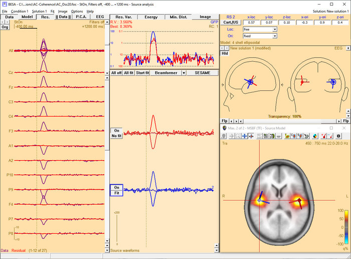
When starting the beamformer from the time-frequency window, a bilateral beamformer scan is performed. In the source analysis window, the beamformer computation can be repeated taking into account possibly correlated sources that are specified in the current solution. Interfering activities generated by all sources in the current solution that are in the 'On' state are specifically suppressed (they enter the matrix L in the beamformer calculation, see Chapter Short mathematical description above). The computation can be started from the Image menu or from the Image selector button dropdown menu. The Image menu can be evoked either from the menu bar or by right-clicking anywhere in the source analysis window.
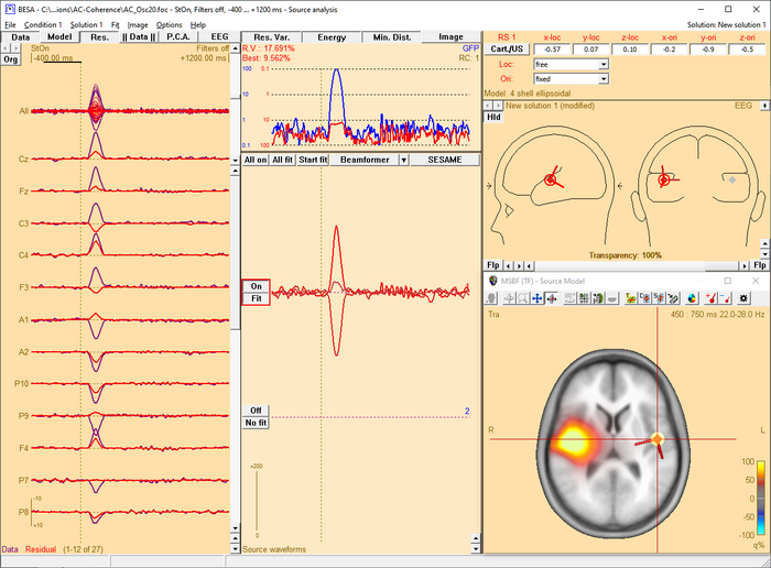
The beamformer scan can be performed with a single or a bilateral source scan. The default scan type depends on the current solution:
- When the beamformer is started from the Time-Frequency window, the Source Analysis window opens with a new solution and a bilateral beamformer scan is performed.
- When the beamformer is started within the Source Analysis window, the default is
- a scan with a single source in addition to the sources in the current solution, if at least one source is active.
- a bilateral scan if no source in the current solution is active.
The default scan type is the multiple source beamformer. The non-default scan type can be enforced using the corresponding Volume Image / Beamformer entry in the Image menu.
Inserting Sources out of the Beamformer Image
The beamformer image can be used to add sources to the current solution. A simple double-click anywhere in the 2D- or 3D-view will generate a non-oriented regional source at the corresponding location. However, a better and easier way to create sources at image maxima and minima is to use the toolbar buttons Switch to Maximum ![]() and Add Source
and Add Source ![]() .
.
Use the Switch to Maximum button to place the red crosshair of the 3D window onto a local image maximum or minimum. Hitting the Add Source button creates a regional source at the location of the crosshair and therefore ensures the exact placement of the source at the image extremum. Moreover, the Add Source button generates an oriented regional source. BESA Research automatically estimates the source orientation that contributes most to the power in the target time-frequency interval (or the reference time-frequency interval, if its power is larger than that in the target interval). The accuracy of this orientation estimate depends largely on the noise content of the data. The smaller the signal-to-noise ratio of the data, the lower is the accuracy of the orientation estimate. This feature allows to use the beamformer as a tool to create a source montage for source coherence analysis, where it is of advantage to work with oriented sources.
Notes:
- You can hide or re-display the last computed image by selecting the corresponding entry in the Image menu.
- The current image can be exported to ASCII or BrainVoyager vmp-format from the Image menu.
- For scaling options, use the
 and
and  Image Scale toolbar buttons.
- Parameters used for the beamformer calculations can be set in the Standard Volumes of the Image Settings dialog box.
Dynamic Imaging of Coherent Sources (DICS)
Short mathematical introduction
Dynamic Imaging of Coherent Sources (DICS) is a sophisticated method for imaging cortico-cortical coherence in the brain, or coherence between an external reference (e.g. EMG channel) and cortical structures. DICS can be applied to localize evoked as well as induced coherent cortical activity in a user-defined time-frequency range.
DICS was implemented in BESA closely following Gross et al., "Dynamic imaging of coherent sources: Studying neural interactions in the human brain", PNAS 98, 694-699, 2001.
The computation is based on a transformation of each channel's single trial data from the time domain into the frequency domain. This transformation is performed by the BESA Research Coherence module and results in the complex spectral density matrix that is used for constructing the spatial filter similar to beamforming.
DICS computation yields a 3-D image, each voxel being assigned a coherence value. Coherence values can be described as a neural activity index and do not have a unit. The neural activity index contrasts coherence in a target time-frequency bin with coherence of the same time-frequency bin in a baseline.
DICS for cortico-cortical coherence is computed as follows:
Let L(r) be the leadfield in voxel r in the brain and C the complex cross-spectral density matrix. The spatial filter W(r) for the voxel r in the head is defined as follows:
[math]W\left( r \right) = \left\lbrack L^{T}\left( r \right) \cdot C^{- 1} \cdot L\left( r \right) \right\rbrack^{- 1} \cdot L^{T}(r) \cdot C^{- 1}[/math]
The cross-spectrum between two locations (voxels) r1 and r2 in the head are calculated with the following equation:
[math]C_{s}\left( r_{1},r_{2} \right) = W\left( r_{1} \right) \cdot C \cdot W^{*T}\left( r_{2} \right),[/math]
where *T means the transposed complex conjugate of a matrix. The cross-spectral density can then be calculated from the cross spectrum as follows:
[math]c_{s}\left( r_{1},r_{2} \right) = \lambda_{1}\left\{ C_{s}\left( r_{1},r_{2} \right) \right\},[/math]
where λ1{} indicates the largest singular value of the cross spectrum. Once the cross spectral density is estimated, the connectivity¹(CON) between the two brain regions r1 and r2 are calculated as follows:
[math]\text{CON}\left( r_{1},r_{2} \right) = \frac{c_{s}^{\text{sig}}\left( r_{1},r_{2} \right) - c_{s}^{\text{bl}}(r_{1},r_{2})}{c_{s}^{\text{sig}}\left( r_{1},r_{2} \right) + c_{s}^{\text{bl}}(r_{1},r_{2})},[/math]
where cssig is the cross-spectral density for the signal of interest between the two brain regions r1 and r2, and csbl is the corresponding cross spectral density for the baseline or the control condition, respectively. In the case DICS is computed with a cortical reference, r1 is the reference region (voxel) and remains constant while r2 scans all the grid points within the brain sequentially. In that way, the connectivity between the reference brain region and all other brain regions is estimated. The value of CON(r1, r2) falls in the interval [-1 1]. If the cross-spectral density for the baseline is 0 the connectivity value will be 1. If the cross-spectral density for the signal is 0 the connectivity value will be -1.
¹ Here, the term connectivity is used rather than coherence, as strictly speaking the coherence equation is defined slightly differently. For simplicity reasons the rest of the tutorial uses the term coherence.
DICS for cortico-muscular coherence is computed as follows:
When using an external reference, the equation for coherence calculation is slightly different compared to the equation for cortico-cortical coherence. First of all, the cross-spectral density matrix is not only computed for the MEG/EEG channels, but the external reference channel is added. This resulting matrix is Call. In this case, the cross-spectral density between the reference signal and all other MEG/EEG channels is called cref. It is only one column of Call. Hence, the cross-spectrum in voxel r is calculated with the following equation:
[math]C_{s}\left( r \right) = W\left( r \right) \cdot c_{\text{ref}}[/math]
and the corresponding cross-spectral density is calculated as the sum of squares of Cs:
[math]c_{s}\left( r \right) = \sum_{i = 1}^{n}{C_{s}\left( r \right)_{i}^{2}},[/math]
where n is 2 for MEG and 3 for EEG. This equation can also be described as the squared Euclidean norm of the cross-spectrum:
[math]c_{s}\left( r \right) = \left\| C_{s} \right\|^{2},[/math]
The power in voxel r is calculated as in the cortico-cortical case:
[math]p\left( r \right) = \lambda_{1}\left\{ C_{s}(r,r) \right\}.[/math]
At last, coherence between the external reference and cortical activity is calculated with the equation:
[math]\text{CON}\left( r \right) = \frac{c_{s}(r)}{p\left( r \right) \cdot C_{\text{all}}(k,k)},[/math]
where Call(k, k) is the (k,k)-th diagonal element of the matrix Call.
DICS is particularly useful, if coherence is to be calculated without an a-priory source model (in contrast to source coherence based on pre-defined source montages). However, the recommended analysis strategy for DICS is to use a brain source as a starting point for coherence calculation that is known to contribute to the EEG/MEG signal of interest. For example, one might first run a beamformer on the time-frequency range of interest and use the voxel with the strongest oscillatory activity as a starting point for DICS. The resulting coherence image will again lead to several maxima (ordered by magnitude), which in turn can serve as starting points for DICS calculation. This way, it is possible to detect even weak sources that show coherent activity in the given time-frequency range.
The other significant application for DICS is estimating coherence between an external source and voxels in the brain. For example, an external source can be muscle activity recoded by an electrode placed over the according peripheral region. This way, the direct relationship between muscle activity and brain activation can be measured.
Starting DICS computation from the Time-Frequency Window
DICS is particularly useful, if coherence in a user-defined time-frequency bin (evoked or induced) is to be calculated between any two brain regions or between an external reference and the brain. DICS runs only on time-frequency decomposed data, so time-frequency analysis needs to be run before starting DICS computation.
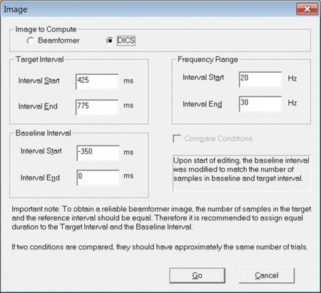
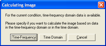
To start the DICS computation, left-drag a window over a selected time-frequency bin in the Time-Frequency Window. Right-click and select “Image”. A dialogue will open (see fig. 1) prompting you to specify time and frequency settings as well as the baseline period. It is recommended to use a baseline period of equal length as the data period of interest. Make sure to select “DICS” in the top row and press “Go”.
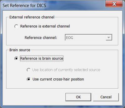
Next, a window will appear allowing you to specify the reference source for coherence calculation (see fig. 2). It is possible to select a channel (e.g. EMG) or a brain source. If a brain source is chosen and no source analysis was computed beforehand, the option “Use current cross-hair position” must be chosen. In case discrete source analysis was computed previously, the selected source can be chosen as the reference for DICS. Please note that DICS can be re-computed with any cross-hair or source position at a later stage.
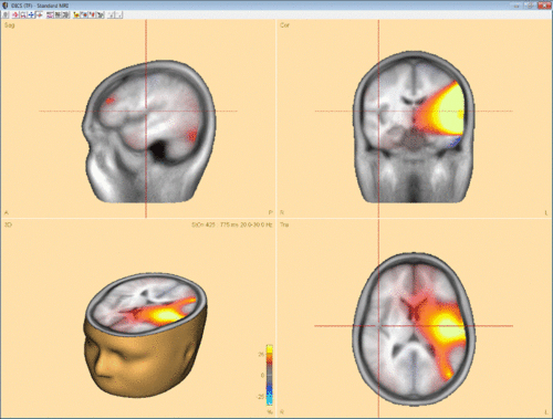
Confirming with “OK” will start computation of coherence between the selected channel/voxel and all other brain voxels. In case DICS is computed for a reference source in the brain, it can be advantageous to run a beamforming analysis in the selected time-frequency window first and use one of the beamforming maxima as reference for DICS. Fig. 3 shows an example for DICS calculation.
Coherence values range between -1 and 1. If coherence in the signal is much larger than coherence in the baseline (control condition) then the DICS value is going to approach 1. Contrary, if coherence in the baseline is much larger than coherence in the signal, then the DICS value is going to approach -1. At last, if coherence in the signal is equal to coherence in the baseline, then the DICS value is 0.
In case DICS is to be re-computed with a different reference, simply mark the desired reference position by placing the cross-hair in the anatomical view and select “DICS” in the middle panel of the source analysis window (see Fig. 4). In case an external reference is to be selected, click on “DICS” in the middle panel to bring up the DICS dialogue (see. Fig. 2) and select the desired channel. Please note that DICS computation will only be available after running time-frequency analysis.
Multiple Source Beamformer (MSBF) in the Time Domain
This feature requires BESA Research 7.0 or higher.
Short mathematical introduction
Beamforming approach can be also applied in the time domain data. This approach was introduced as linearly constrained minimum variance (LCMV) beamformer (Van Veen et al., 1997). It allows to image evoked activity in a user-defined time range, where time is taken relative to a triggered event, and to estimate source waveforms using the calculated spatial weight at locations of interest. For an implementation of the beamformer in the time domain, data covariance matrices are required, while complex cross spectral density matrices are used for the beamformer approaches in the time-frequency domain as described in the Multiple Source Beamformer (MSBF) in the Time-frequency Domain section.
The bilateral beamformer introduced in the Multiple Source Beamformer (MSBF) in the Time-frequency Domain section is also implemented for the time-domain beamformer to take into account contributions from the homologue source in the opposite. This allows for imaging of highly correlated bilateral activity in the two hemispheres that commonly occurs during processing of external stimuli. In addition, the beamformer computation can take into account possibly correlated sources at arbitrary locations.
The beamformer spatial weight W(r) for the voxel r in the brain is defined as follows (Van Veen et al., 1997):
[math]\mathrm{W}(r) = [\mathrm{L}^T(r)\mathrm{C}^{-1}\mathrm{L}(r)]^{-1}\mathrm{L}^T(r)\mathrm{C}^{-1}[/math]
where [math]\mathrm{C}^{-1}[/math] is the inversed regularized average of covariance matrix over trials, L is the leadfield matrix of the model containing a regional source at target location r and optionally additional sources whose interference with the target source is to be minimized. The beamformer spatial weight W(r) can be applied to the measured data to estimate source waveform at a location r (beamformer virtual sensor):
[math]\mathrm{S}(r,t) = \mathrm{W}(r)\mathrm{M}(t)[/math]
where S(r,t) represents the estimated source waveform and M(t) represents measured EEG or MEG signals. The output power P of the beamformer for a specific brain region at location r is computed by the following equation:
[math]\mathrm{P}(r) = \operatorname{tr^{'}}[\mathrm{W}(r) \cdot \mathrm{C} \cdot \mathrm{W}^T(r)][/math]
where tr’[ ] is the trace of the [3×3] (MEG: [2×2]) submatrix of the bracketed expression that corresponds to the source at target location r.
Beamformer can suppress noise sources that are correlated across sensors. However, uncorrelated noise will be amplified in a spatially non-uniform manner, with increasing distortion with increasing distance from the sensors (Van Veen et al., 1997; Sekihara et al., 2001). For this reason, estimated source power should be normalized by a noise power. In BESA Research, the output power P(r) is normalized with the output power in a baseline interval or with the output power of a uncorrelated noise: P(r) / Pref (r).
The time-domain beamformer image is constructed from values q(r) computed for all locations on a grid specified in the General Settings tab. A value q(r) is defined as described in the Multiple Source Beamformer (MSBF) in the Time-frequency Domain section with data covariance matrices instead of cross-spectral density matrices.
Applying the Beamformer
This chapter illustrates the usage of the BESA beamformer in the time domain. The displayed figures are generated using the file ‘Examples/ERP-Auditory-Intensity/S1.cnt’.
Starting the time-domain beamformer from the Average tab of the Paradigm dialog box
The time-domain beamformer is needed data covariance matrices and therefore requires the ERP module to be enabled. After the beamformer computation has been initiated in the Average tab of the Paradigm dialog box, the source analysis window opens with an enlarged 3D image of the q-value computed with a bilateral beamformer. The result is superimposed onto the MR image assigned to the data set (individual or standard).
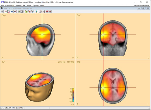
Multiple-source beamformer in the Source Analysis window
The 3D imaging display is part of the source analysis window. In the Channel box, the averaged (evoked) data of the selected condition is shown. Selected covariance intervals in the ERP module can be checked in the Channel box. The red, gray, and blue rectangles indicate signal, baseline, and common interval, respectively.
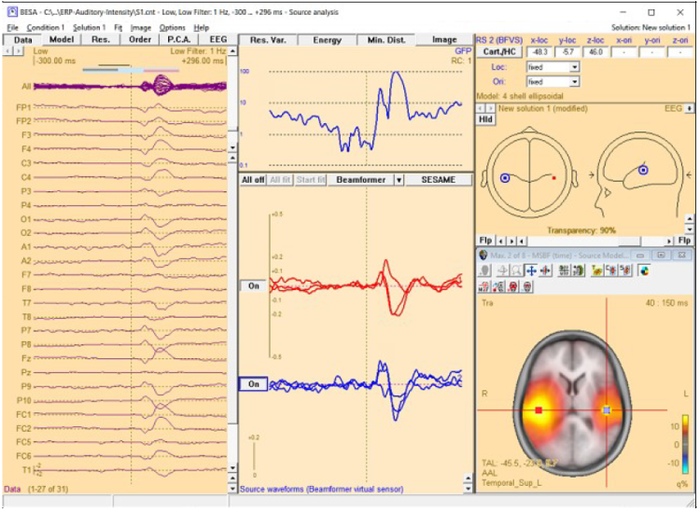
When starting the beamformer from the Average tab of the Paradigm dialog box, the bilateral beamformer scan is performed. In the source analysis window, the beamformer computation can be repeated taking into account possibly correlated sources that are specified in the current solution. Interfering activities generated by all sources in the current solution that are in the 'On' state are specifically suppressed (they enter the leadfield matrix L in the beamformer calculation). The computation can be started from the Image menu or from the Image selector button ![]() dropdown menu. The Image menu can be evoked either from the menu bar or by right-clicking anywhere in the source analysis window.
dropdown menu. The Image menu can be evoked either from the menu bar or by right-clicking anywhere in the source analysis window.
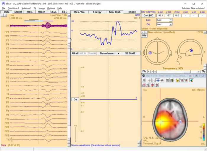
The beamformer scan can be performed with a single or a bilateral source scan. The default scan type depends on the current solution:
When the beamformer is started from the Average tab of the Paradigm dialog box the Source Analysis window opens with a new solution and a bilateral beamformer scan is performed.
When the beamformer is started within the Source Analysis window, the default is:
- a scan with a single source in addition to the sources in the current solution, if at least one source is active.
- a bilateral scan if no source in the current solution is active.
- a scan with a single source when scalar-type beamformer is selected in the beamformer option dialog box.
The default scan type is the multiple source beamformer. The non-default scan type can be enforced using the corresponding Volume Image / Beamformer entry in the Image main menu or in the beamformer option dialog box (only for the time-domain beamformer).
Inserting Sources as Beamformer Virtual Sensor out of the Beamformer Image
This is similar to the inserting sources out of the beamformer image in Multiple Source Beamformer (MSBF) in the Time-frequency Domain section.
The beamformer image can be used to add beamformer virtual sensors to the current solution. A simple double-click anywhere in the 3D view (not in the 2D view) will generate a source at the corresponding location. A better and easier way to create sources at image maxima and minima is to use the toolbar buttons Switch to Maximum ![]() and Add Source
and Add Source ![]() .
.
This feature allows to use the beamformer as a tool to create a source montage for source coherence analysis. A source montage file (*.mtg) for beamformer virtual sensors can be saved using File \ Save Source Montage As… entry.
The time-domain beamformer image can be also used to add regional or dipole sources to the current solution. Press N key when there is no source in the current source array or there is more than one beamformer virtual sensor. To create a new source array for beamformer virtual sensor, press N key when there is more than one regional or dipole source in the current source array.
Notes
- You can hide or re-display the last computed image by selecting Hide Image entry in the Image menu.
- The current image can be exported to ASCII, ANALYZE, or BrainVoyager (*.vmp) format from the Image menu.
- For scaling options, use
 and
and  Image Scale toolbar buttons.
- Parameters used for the beamformer calculations can be set in the Standard Volume tab of the Image Settings dialog box.
- Note that Model, Residual, Order, and Residual variance are not shown for the beamformer virtual sensor type sources.
References
- Sekihara, K., Nagarajan, S. S., Poeppel, D., Marantz, A., & Miyashita, Y. (2001). Reconstructing spatio-temporal activities of neural sources using an MEG vector beamformer technique. IEEE Transactions on Biomedical Engineering, 48(7), 760–771.
- Van Veen, B. D., Van Drongelen, W., Yuchtman, M., & Suzuki, A. (1997). Localization of brain electrical activity via linearly constrained minimum variance spatial filtering. IEEE Transactions on Biomedical Engineering, 44(9), 867–880
CLARA
CLARA ('Classical LORETA Analysis Recursively Applied') is an iterative application of weighted LORETA images with a reduced source space in each iteration.
In an initialization step, a LORETA image is calculated. Then in each iteration the following steps are performed:
- The obtained image is spatially smoothed (this step is left out in the first iteration).
- All grid points with amplitudes below a threshold of 1% of the maximum activity are set to zero, thus being effectively eliminated from the source space in the following step.
- The resulting image defines a spatial weighting term (for each voxel the corresponding image amplitude).
- A LORETA image is computed with an additional spatial weighting term for each voxel as computed in step 3. By the default settings in BESA Research, the regularization values used in the iteration steps are slightly higher than that of the initialization LORETA image.
The procedure stops after 2 iterations, and the image computed in the last iteration is displayed. Please note that you can change all parameters by creating a user-defined volume image.
The advantage of CLARA over non-focusing distributed imaging methods is visualized by the figure below. Both images are computed from the N100 response in an auditory oddball experiment (file Oddball.fsg in subfolder fMRI+EEG-RT-Experiment of the Examples folder). The CLARA image is much more focal than the sLORETA image, making it easier to determine the location of the image maxima.
Notes:
- Starting CLARA: CLARA can be started from the Image menu or from the Image Selection button.
- Please refer to Chapter Regularization of distributed volume images for important information on regularization of distributed inverses.
LAURA
LAURA (Local Auto Regressive Average) belongs to the distributed inverse method of the family of weighted minimum norm methods (Grave de Peralta Menendeza et al., "Noninvasive Localization of Electromagnetic Epileptic Activity. I. Method Descriptions and Simulations", BrainTopography 14(2), 131-137, 2001). LAURA uses a spatial weighting function that includes depth weighting and that term has the form of a local autoregressive function.
The source activity is estimated by applying the general formula for a weighted minimum norm:
[math]\mathrm{S}\left( t \right) = \mathrm{V} \cdot \mathrm{L}^{T}\left( \mathrm{L} \cdot \mathrm{V} \cdot \mathrm{L}^{T} \right)^{- 1} \cdot \mathrm{D}(t)[/math]
Here, L is the leadfield matrix of the distributed source model with regional sources distributed on a regular cubic grid. D(t) is the data at time point t. The term in parentheses is generally regularized. Regularization parameters can be specified in the Image Settings.
In LAURA, V contains both a depth weighting term W and a representation of a local autoregressive function A. V is computed as:
[math]\mathrm{V} = \left( \mathrm{U}^{T} \cdot \mathrm{U} \right)^{-1}[/math]
where
[math]\mathrm{U} = \left( \mathrm{W} \cdot \mathrm{A} \right) \otimes \mathrm{I}_{3}[/math]
Here, [math]\otimes[/math] denotes the Kronecker product. I3 is the [3×3] identity matrix. W is an [s×s] diagonal matrix (with s the number of source locations on the grid), where each diagonal element is the inverse of the maximum singular value of the corresponding regional source's leadfields. The formula for the diagonal components Aii and the off-diagonal components Aik are as follows:
[math]\mathrm{A}_{ii} = \frac{26}{\mathrm{N}_{i}}\sum_{k \subset V_{i}}^{}\frac{1}{\mathrm{d}_{ik}^{2}}[/math]
[math] \mathrm{A}_{ik} = \begin{cases} - 1/\operatorname{dist}\left( i,k \right)^{2}, & \text{if } k \subset V_{i} \\ 0, & \text{otherwise} \end{cases} [/math]
Here, Vi is the vicinity around grid point i that includes the 26 direct neighbors.
The LAURA image in BESA Research displays the norm of the 3 components of S at each location r. Using the menu function Image / Export Image As... you have the option to save this norm of S or alternatively all components separately to disk.
Notes:
- Grid spacing: Due to memory limitations, LAURA images require a grid spacing of 7 mm or more.
- Computation time: Computation speed during the first LAURA image calculation depends on the grid spacing (computation is faster with larger grid spacing). After the first computation of a LAURA image, a *.laura file is stored in the data folder, containing intermediate results of the LAURA inverse. This file is used during all subsequent LAURA image computations. Thereby, the time needed to obtain the image is substantially reduced.
- MEG: In the case of MEG data, an additional constraint is implemented in the LAURA algorithm that prevents solutions from containing radial source currents (compare Pascual-Marqui, ISBET Newsletter 1995, 22-29). In MEG, an additional source space regularization is necessary in the inverse matrix operation required compute V
- Starting LAURA: LAURA can be started from the Image menu or from the Image Selection button.
- Regularization: Please refer to Chapter “Regularization of distributed volume images” for important information on regularization of distributed inverses.
LORETA
LORETA ("Low Resolution Electromagnetic Tomography") is a distributed inverse method of the family of weighted minimum norm methods. LORETA was suggested by R.D. Pascual-Marqui (International Journal of Psychophysiology. 1994, 18:49-65). LORETA is characterized by a smoothness constraint, represented by a discrete 3D Laplacian.
The source activity is estimated by applying the general formula for a weighted minimum norm:
[math]\mathrm{S}\left( t \right) = \mathrm{V} \cdot \mathrm{L}^{T}\left( \mathrm{L} \cdot \mathrm{V} \cdot \mathrm{L}^{T} \right)^{- 1} \cdot \mathrm{D}(t)[/math]
Here, L is the leadfield matrix of the distributed source model with regional sources distributed on a regular cubic grid. D(t) is the data at time point t. The term in parentheses is generally regularized. Regularization parameters can be specified in the Image Settings.
In LORETA, V contains both a depth weighting term and a representation of the 3D Laplacian matrix. V is computed as:
[math]\mathrm{V} = \left( \mathrm{U}^{T} \cdot \mathrm{U} \right)^{- 1}[/math]
where
[math]\mathrm{U} = \left( \mathrm{W} \cdot \mathrm{A} \right) \otimes \mathrm{I}_{3}[/math]
Here, [math]\otimes[/math] denotes the Kronecker product. I3 is the [3x3] identity matrix. W is an [sxs] diagonal matrix (with s the number of source locations on the grid), where each diagonal element is the inverse of the maximum singular value of the corresponding regional source's leadfields. A contains the 3D Laplacian and is computed as
[math]\mathrm{A} = \mathrm{Y} - \mathrm{I}_{s}[/math]
with Is the [sxs] identity matrix, where s is the number of sources (= three times the number of grid points) and
[math]\mathrm{Y} = \frac{1}{2}\left\{ \mathrm{I}_{s} + \left\lbrack \operatorname{diag}\left( \mathrm{Z} \cdot \left\lbrack 111 \ldots 1 \right\rbrack^{T} \right) \right\rbrack^{- 1} \right\} \cdot \mathrm{Z}[/math]
where
[math]
\mathrm{Z}_{ik} =
\begin{cases}
1/6, & \text{if } \operatorname{dist}\left( i,k \right) = 1 \text{ grid point} \\
0, & \text{otherwise}
\end{cases}
[/math]
The LORETA image in BESA Research displays the norm of the 3 components of S at each location r. Using the menu function Image / Export Image As... you have the option to save this norm of S or alternatively all components separately to disk.
Notes:
- Grid spacing: Due to memory limitations, LORETA images require a grid spacing of 5 mm or more.
- Computation time: Computation speed during the first LORETA image calculation depends on the grid spacing (computation is faster with larger grid spacing). After the first computation of a LORETA image, a *.loreta file is stored in the data folder, containing intermediate results of the LORETA inverse. This file is used during all subsequent LORETA image computations. Thereby, the time needed to obtain the image is substantially reduced.
- MEG: In the case of MEG data, an additional constraint is implemented in the LORETA algorithm that prevents solutions from containing radial source currents (Pascual-Marqui, ISBET Newsletter 1995, 22-29). In MEG, an additional source space regularization is necessary in the inverse matrix operation required compute V.
- Starting LORETA: LORETA can be started from the Image menu or from the Image Selection button.
- Regularization: Please refer to Chapter “Regularization of distributed volume images” for important information on regularization of distributed source models.
sLORETA
This distributed inverse method consists of a standardized, unweighted minimum norm. The method was originally suggested by R.D. Pascual-Marqui (Methods & Findings in Experimental & Clinical Pharmacology 2002, 24D:5-12) Starting point is an unweighted minimum norm computation:
[math]\mathrm{S}_{\text{MN}}\left( t \right) = \mathrm{L}^{T} \cdot \left( \mathrm{L} \cdot \mathrm{L}^{T} \right)^{- 1} \cdot \mathrm{D}(t)[/math]
Here, L is the leadfield matrix of the distributed source model with regional sources distributed on a regular cubic grid. D(t) is the data at time point t. The term in parentheses is generally regularized. Regularization parameters can be specified in the Image Settings.
This minimum norm estimate is now standardized to produce the sLORETA activity at a certain brain location r:
[math]\mathrm{S}_{\text{sLORETA}, r} = \mathrm{R}_{rr}^{-1/2} \cdot \mathrm{S}_{\text{MN},r}[/math]
SsMN,r is the [3x1] (MEG: [2x1]) minimum norm estimate of the 3 (MEG: 2) dipoles at location r. Rrr is the [3x3] (MEG: [2x2]) diagonal block of the resolution matrix R that corresponds to the source components at the target location r. The resolution matrix is defined as:
[math]\mathrm{R} = \mathrm{L}^{T} \cdot \left( \mathrm{L} \cdot \mathrm{L}^{T} + \lambda \cdot \mathrm{I} \right)^{-1} \cdot \mathrm{L}[/math]
The sLORETA image in BESA Research displays the norm of SsLORETA, r at each location r. Using the menu function Image / Export Image As... you have the option to save this norm of SsLORETA, r or alternatively all components separately to disk.
Notes:
- sLORETA can be started from the Image menu or from the Image Selection button.
- Please refer to Chapter Regularization of distributed volume images for important information on regularization of distributed inverses.
swLORETA
This distributed inverse method is a standardized, depth-weighted minimum norm (E. Palmero-Soler et al 2007 Phys. Med. Biol. 52 1783-1800). It differs from sLORETA only by an additional depth weighting.
Starting point is a depth-weighted minimum norm computation:
[math]\mathrm{S}_{\text{MN}}\left( t \right) = \mathrm{V} \cdot \mathrm{L}^{T} \cdot \left( \mathrm{L} \cdot \mathrm{V} \cdot \mathrm{L}^{T} \right)^{-1} \cdot \mathrm{D}(t)[/math]
Here, L is the leadfield matrix of the distributed source model with regional sources distributed on a regular cubic grid. D(t) is the data at time point t. The term in parentheses is generally regularized. Regularization parameters can be specified in the Image Settings.
V is the diagonal depth weighting matrix. For s grid locations, V is of dimension [3s x 3s] (MEG: [2s x 2s]). Each diagonal element of V is the inverse of the first singular value of the leadfield of the corresponding regional source. Hence, the first 3 (MEG: 2) diagonal elements equal the inverse of the largest eigenvalue of the leadfield matrix of regional source 1, and so on.
This minimum norm estimate is now standardized to produce the swLORETA activity at a certain brain location r:
[math]\mathrm{S}_{\text{swLORETA},r} = \mathrm{R}_{rr}^{-1/2} \cdot \mathrm{S}_{\text{MN},r}[/math]
SsMN,r is the [3x1] (MEG: [2x1]) depth-weighted minimum norm estimate of the regional source at location r. Rrr is the [3x3] (MEG: [2x2]) diagonal block of the resolution matrix R that corresponds to the source components at the target location r. The resolution matrix is defined as:
[math]\mathrm{R} = \mathrm{V} \cdot \mathrm{L}^{T} \cdot \left( \mathrm{L} \cdot \mathrm{V} \cdot \mathrm{L}^{T} + \lambda \cdot \mathrm{I} \right)^{-1} \cdot \mathrm{L}[/math]
The swLORETA image in BESA Research displays the norm of SswLORETA, r at each location r. Using the menu function Image / Export Image As... you have the option to save this norm of SswLORETA, r or alternatively all components separately to disk.
Notes:
- sLORETA can be started from the Image menu or from the Image Selection button.
- Please refer to Chapter “Regularization of distributed volume images” for important information on regularization of distributed inverses.
sSLOFO
SSLOFO (standardized shrinking LORETA-FOCUSS) is an iterative application of weighted distributed source images with a reduced source space in each iteration (Liu et al., "Standardized shrinking LORETA-FOCUSS (SSLOFO): a new algorithm for spatio-temporal EEG source reconstruction", IEEE Transactions on Biomedical Engineering 52(10), 1681-1691, 2005).
In an initialization step, an sLORETA image is calculated. Then in each iteration the following steps are performed:
- A weighted minimum norm solution is computed according to the formula [math]\mathrm{S} = \mathrm{V} \cdot \mathrm{L}^{T} \cdot \left( \mathrm{L} \cdot \mathrm{V} \cdot \mathrm{L}^{T} \right)^{-1} \cdot \mathrm{D}[/math] . Here, L is the leadfield matrix of the distributed source model with regional sources distributed on a regular cubic grid. D is the data at the time point under consideration. V is a diagonal spatial weighting matrix that is computed in the previous iteration step. In the first iteration, the elements of V contain the magnitudes of the initially computed LORETA image.
- Standardization of this weighted minimum norm image is performed with the resolution matrix as in sLORETA.
- The obtained standardized weighted minimum norm image is being smoothed to get Ssmooth.
- All voxels with amplitudes below a threshold of 1% of the maximum activity get a weight of zero in the next iteration step, thus being effectively eliminated from the source space in the next iteration step.
- For all other voxels, compute the elements of the spatial weighting matrix V to be used in the next iteration as follows: [math]\mathrm{V}_{ii,\text{next iteration}} = \frac{1}{\left\| \mathrm{L}_{i} \right\|} \cdot \mathrm{S}_{ii,\text{smooth}} \cdot \mathrm{V}_{ii,\text{current iteration}}[/math]
The procedure stops after 3 iterations. Please note that you can change all parameters by creating a user-defined volume image.
Notes:
- Starting sSLOFO: sSLOFO can be started from the Image menu or from the Image Selection button.
- Please refer to Chapter Regularization of distributed volume images for important information on regularization of distributed inverses.
User-Defined Volume Image
In addition to the predefined 3D imaging methods in BESA Research, it is possible to create user-defined imaging methods based on the general formula for distributed inverses:
[math]\mathrm{S}\left( t \right) = \mathrm{V} \cdot \mathrm{L}^{T} \cdot \left( \mathrm{L} \cdot \mathrm{V} \cdot \mathrm{L}^{T} \right)^{-1} \cdot \mathrm{D}(t)[/math]
Here, L is the leadfield matrix of the distributed source model with regional sources distributed on a regular cubic grid. D(t) is the data at time point t. Custom-defined parameters are:
- The spatial weighting matrix V: This may include depth weighting, image weighting, or cross-voxel weighting with a 3D Laplacian (as in LORETA) or an autoregressive function (as in LAURA).
- Regularization: The term in parentheses is generally regularized. Note that regularization has a strong effect on the obtained results. Please refer to chapter Regularization of Distributed Volume Imagesfor more information.
- Standardization: Optionally, the result of the distributed inverse can be standardized with the resolution matrix (as in sLORETA).
- Iterations: Inverse computations can be applied iteratively. Each iteration is weighted with the image obtained in the previous iteration.
All parameters for the user-defined volume image are specified in the User-Defined Volume Tab of the Image Settings dialog box. Please refer to chapter User-Defined Volume Tab for details.
Notes:
- Starting the user-defined volume image: the image calculation can be started from the Image menu or from the Image Selection button.
- Please refer to Chapter Regularization of distributed volume images for important information on regularization of distributed inverses.
Regularization of distributed volume images
Distributed source images require the inversion of a term of the form L V LT. This term is generally regularized before its inversion. In BESA Research, selection can be made between two different regularization approaches (parameters are defined in the Image Settings dialog box):
- Tikhonov regularization: In Tikhonov regularization, the term L V LT is inverted as (L V LT +λ I)-1. Here, l is the regularization constant, and I is the identity matrix.
- One way of determining the optimum regularization constant is by minimizing the generalized cross validation error (CVE).
- Alternatively, the regularization constant can be specified manually as a percentage of the trace of the matrix L V LT.
- TSVD: In the truncated singular value decomposition (TSVD) approach, an SVD decomposition of L V LT is computed as L V LT = U S UT, where the diagonal matrix S contains the singular values. All singular values smaller than the specified percentage of the maximum singular values are set to zero. The inverse is computed as U S-1 UT, where the diagonal elements of S-1 are the inverse of the corresponding non-zero diagonal elements of S.
Regularization has a critical effect on the obtained distributed source images. The results may differ completely with different choices of the regularization parameter (see examples below). Therefore, it is important to evaluate the generated image critically with respect to the regularization constant, and to keep in mind the uncertainties resulting from this fact when interpreting the results. The default setting in BESA Research is a TSVD regularization with a 0.03% threshold. However, this value might need to be adjusted to the specific data set at hand.
The following example illustrates the influence of the regularization parameter on the obtained images. The data used here is condition St-Cor of dataset Examples \ TFC-Error-Related-Negativity \ Correct+Error.fsg at 176 ms following the visual stimulus. Discrete dipole analysis reveals the main activity in the left and right lateral visual cortex at this latency.
LORETA images computed at this latency depend critically on the choice of the regularization constant. The following 3D images are created with TSVD regularization with SVD cutoffs of 0.1%, 0.005%, and 0.0001%, respectively. The volume grid size was 9 mm. The example demonstrates the dramatic effect of regularization and demonstrates the typical tradeoff between too strong regularization (leading to too smeared 3D images that tend to show blurred maxima) and too small regularization (resulting in too superficial 3D images with multiple maxima).
The automatic determination of the regularization constant using the CVE approach does not necessarily result in the optimum regularization parameter either. In this example, the unscaled CVE approach rather resembles the TSVD image with a cutoff of 0.0001%, i.e. regularization is too small. Therefore, it is advisable to compare different settings of the regularization parameter and make the final choice based on the above-mentioned considerations.
Cortical LORETA
Cortical LORETA is principally the same technique as LORETA, however, Cortical LORETA is not computed in a 3D volume, but on the cortical surface.
The cortical reconstruction in BESA Research fed from BESA MRI is a closed 2D surface with no boundaries and a very close approximation of the actual cortical form. It consists of an irregular triangulated grid.
The Laplace operator that is used for identifying a smooth solution in a three-dimensional space is exchanged with a Laplace operator that runs on the two-dimensional cortical surface.
There is a wide variety of 2D Laplace operators with different characteristics. The general form of the discrete Laplace operator is
[math]\Delta f\left( p_{i} \right) = \frac{1}{d_{i}}\sum_{j \in N(i)}^{}{w_{ij}\left\lbrack f\left( p_{i} \right) - f\left( p_{j} \right) \right\rbrack},[/math]
where pi is the i-th node of the triangular mesh, f(pi) is the value of a function f defined on the cortical mesh at the node pi, wij is the weight for the connection between the nodes pi and pj and di is a normalization factor for the i-th row of the operator. Furthermore, N(i) is the set of indices corresponding to the direct (also called "1-ring") neighbors of pi.
BESA offers the choice of three Laplace operators with slightly different characteristics.
- Unweighted Graph Laplacian: This is the simplest operator. It takes into account only the adjacency of the nodes and not the geometry of the mesh:
[math]
w_{ij} =
\begin{cases}
1, & \text{if } p_{i} \text{ and } p_{j} \text{ are connected by an edge} \\
0, & \text{otherwise}
\end{cases}
[/math]
[math]d_{i} = 1[/math]
- Weighted Graph Laplacian: This operator is similar to the unweighted graph Laplacian but with different weights for the different connections. The connections between nearby nodes get larger weights than the connections between farther nodes:
[math]w_{ij} = \frac{1}{\operatorname{dist}\left( p_{i},p_{j} \right)}[/math]
[math]d_{i} = \sum_{j \in N(i)}^{} {\operatorname{dist}\left(p_{i}, p_{j} \right)}[/math]
where dist (pi , pj) is the distance between the nodes pi and pj.
- Geometric Laplacian with mixed area weights: This operator takes into account the angles in the corresponding triangles into account as well as the area around the nodes in order to determine the connection weights:
[math]w_{ij} = \frac{\cot\left( \alpha_{ij} \right) + \cot\left( \beta_{ij} \right)}{2}[/math]
[math]d_{i} = A_{\text{mixed}}[/math]
where αij and βij denote the two angles opposite to the edge (i , j) and Amixed is either the Voronoi area, or 1/2 of the triangle area or 1/4 of the triangle area depending on the type of the triangle.
Regularization and other parameters:
- SVD cutoff: The regularization for the inverse operator as a percent of the largest singular value.
- Depth weighting: Turn depth weighting on or off.
- Laplacian type: Selection of Laplacian operators (see above).
Notes:
- Starting Cortical LORETA: Cortical LORETA can be started from the sub-menu Surface Image of the Image menu or from the Image Selection button.
- Please refer to Chapter “Regularization of distributed volume images” for important information on regularization of distributed inverses.
References:
Please refer to Iordanov et al.: LORETA With Cortical Constraint: Choosing an Adequate Surface Laplacian Operator. Front Neurosci 12, Article 746, 2018, for more information - full article available here.
Cortical CLARA
Cortical CLARA is principally the same technique as CLARA, but Cortical CLARA is not computed in a 3D volume, but on the cortical surface. Instead of using a LORETA image as the basis for the iterative application, cortical CLARA uses cortical LORETA.
Regularization and other parameters:
- SVD cutoff: The regularization for the inverse operator as a percent of the largest singular value.
- Depth weighting: Turn depth weighting on or off.
- Laplacian type: Selection of Laplacian operators (see Cortical LORETA).
- No of iterations: Number of iterations for CLARA. The more iterations are used, the sparser becomes the solution.
- Automatic: The algorithm tries to determine the number of iterations automatically. The goodness of fit (GOF) is calculated after every iteration and if there is a big jump in the GOF then the algorithm will stop. If no jumps appear during the calculations then CLARA iterates until the specified number of iterations is reached.
- Regularize iterations: If one wants to use different regularization for the CLARA iterations than the value specified as "SVD cutoff", this option should be selected.
- Amount to clip from img (%): Cortical CLARA uses the solution from the previous iteration as an additional weighting matrix for the current iteration. That weighting matrix is constructed by cutting the "low" activity from the solution. This number specifies how much of the activity should be cut from the previous solution in order to construct the weighting matrix. This value is given as a percentage of the maximal activity. Default value is 10%.
Notes:
- Starting Cortical CLARA: Cortical CLARA can be started from the sub-menu Surface Image of the Image menu or from the Image Selection button.
- Please refer to Chapter “Regularization of distributed volume images” for important information on regularization of distributed inverses.
Cortex Inflation
The inflated cortex is a smoothened version of the individual cortical surface with minimal metric distortions (Fischl, B. et al. (1999). Cortical Surface-Based Analysis: II: Inflation, Flattening, and a Surface-Based Coordinate System. NeuroImage, 9(2), 195–207). Gyri and sulci are smoothened out. The original distances between each point on the cortex and its neighbors are, however, mostly preserved.
Cortical LORETA map overlaid on top of the inflated cortical surface.
A lighter gray color overlaid on top of the surface image indicates the location of a gyrus of the individual cortex surface, while a darker gray color indicates the location of a sulcus. The inflated cortical surface can be computed in BESA MRI 2.0. For more details please refer to the BESA MRI 2.0 help.
Surface Minimum Norm Image
Introduction
The minimum norm approach is a common method to estimate a distributed electrical current image in the brain at each time sample (Hämäläinen & Ilmoniemi 1984). The source activities of a large number of regional sources are computed. The sources are evenly distributed using 1500 standard locations 10% and 30% below the smoothed standard brain surface (when using the standard MRI) or using between 3000-4000 locations on the individual brain surface defined by the gray-white-matter boundary.
Since the number of sources is much larger than the number of sensors in a minimum norm solution, the inverse problem is highly underdetermined and must be stabilized by a mathematical constraint, the minimum norm. Out of the many current distributions that can account for the recorded sensor data, the solution with the minimum L2 norm, i.e. the minimum total power of the current distribution is displayed in BESA Research.
First, the forward solution (leadfield matrix L) of all sources is calculated in the current head model. Then, the source activities S(t) of all source components are computed from the data matrix D(t) using an inverse regularized by the estimated noise covariance matrix:
[math]\mathrm{S}\left( t \right) = \mathrm{R} \cdot \mathrm{L}^{T} \cdot \left( \mathrm{L} \cdot \mathrm{R} \cdot \mathrm{L}^{T} + \mathrm{C}_N \right)^{-1} \cdot \mathrm{D}(t)[/math]
Here, L is the leadfield matrix of the distributed regional source model, CN denotes the noise correlation matrix in sensor space, and R is a weighting matrix in source space. R and CN can be designed in different ways in order to optimize the minimum norm result. The total activity of each regional source is computed as the root mean square of the source activities S(t) of its 3 (MEG:2) components. This total source activity is transformed to a color-coded image of the brain surface. (When the standard brain is used, two sources are assigned to each surface location, located 10% and 30% below the surface, respectively. The color that is displayed on the standard brain surface is the larger of the two corresponding source activities.)
Weighting options
The minimum norm current imaging techniques of BESA Research provide different weighting strategies. Two weighting approaches are available: Depth weighting and spatio-temporal approaches.
- Depth weighting: Without depth weighting, deep sources appear very smeared in a minimum-norm reconstruction. With depth weighting, both deep and superficial sources produce a similar, more focal result. If this weighting method is selected, the leadfield of each regional source is scaled with the largest singular value of the SVD (singular value decomposition) of the source's leadfield.
- Spatio-temporal weighting: Spatio-temporal weighting tries to assign large weight to sources that are assumed to be more likely to contribute to the recorded data.
- Subspace correlation after single source scan: This method divides the signal into a signal and a noise subspace. The correlation of the leadfield of a regional source i with the signal subspace (pi) is computed to find out if the source location contributes to the measured data. The weighting matrix R becomes a diagonal matrix. Each of the three (MEG: 2) components of a regional source get the same weighting value pi2. This approach is based on the signal subspace correlation measure introduced by J.C. Mosher, R. M. Leahy (Recursive MUSIC: A Framework for EEG and MEG Source Localization, IEEE Trans. On Biomed. Eng. Vol. 45, No. 11, November 1998)
- Dale & Sereno 1993: In the approach of Dale and Sereno (J Cogn Neurosci, 1993, 5: 162-176) a signal subspace needs not be defined. The correlation pi of the leadfield of regional source i with the inverse of the data covariance matrix is computed along with the largest singular value λmax of the data covariance matrix. The weighting matrix R is a diagonal matrix with weights:
 . Each of the three (MEG: 2) components of a regional source receives the same weighting value.
Noise regularization
Three methods to estimate the channel noise correlation matrix CN are provided by the program:
- Use baseline: Select this option to estimate the noise from the user-definable baseline. The signal is computed from the data at non-baseline latencies.
- Use 15% lowest values: The baseline activity is computed from the data at those 15% of all displayed latencies that have the lowest global field power. The signal is computed from all displayed latencies.
- Use the full baseline covariance matrix: This option is only available if a previous beamformer image in the time-domain was calculated. In this case, it can be selected from the general image settings dialog tab. The baseline covariance interval is the one selected for the beamformer, and is indicated by a thin horizontal bar in the channel box.
In each case, the activity (noise or signal, respectively) is defined as root-mean-square across all respective latencies for each channel.
The noise covariance matrix CN is constructed as a diagonal matrix. The entries in the main diagonal are proportional to the noise activity of the individual channels (if selected) or are all equally proportional to the average noise activity over all channels. The noise covariance matrix CN is then scaled such that the ratio of the Frobenius norms of the weighted leadfield projector matrix (LRLT) and the noise covariance matrix CN equals the Signal-to-Noise ratio. This scaling can be multiplied by an additional factor (default=1) to sharpen (<1) or smoothen (>1) the minimum norm image.
Applying the Minimum Norm Image
The minimum-norm algorithm is started via the Surface minimum norm image dialog box, which is opened from the Image menu, or by typing the shortcut Ctrl-M: Please refer to Chapter “Surface Minimum Norm Tab” for more details.
As opposed to the other 3D images available from the Image menu, the surface minimum norm image is not computed on a volumetric grid, but rather for locations on the brain surface. Accordingly, the results of the minimum norm image are displayed superimposed to the brain surface mesh rather than to the volumetric MR image.
The figure below shows a minimum norm image computed from the file Examples\Epilepsy\Spikes\Spikes-Child4_EEG+MEG_averaged.fsg. The EEG spike peak was imaged using the individual brain surface of the subject. A baseline from -300 to -70 ms was used. Minimum norm was computed with depth weighting, Spatio-temporal weighting according to Dale & Sereno 1993 and individual noise weighting with a noise scale factor of 0.01. The minimum norm image reveals the location of the spike generator in the close vicinity of the frontal left-hemispheric lesion in this subject.
Multiple Source Probe Scan (MSPS)
Introduction
The MSPS function provides a tool for the validation of a given solution. It is based on the following theoretical consideration: If the recorded EEG/MEG data has been modeled adequately, i.e. all active brain regions are represented by a source in the current solution, then any additional probe source added to the solution will not show any activity apart from noise. The only exception occurs if this probe source is placed in close vicinity to one of the sources in the current solution. In that case, the solution's source and the probe source will share the activity of the corresponding brain area. The MSPS applies these considerations by scanning the brain on a pre-defined grid with a regional probe added to the current solution. Grid extent and density can be specified in the Image settings. The power P of the probe source at location r in the signal interval is compared with the power of the probe source in a reference interval, defining a value q:
[math]\mathrm{q}\left( r \right) = \sqrt{\frac{\mathrm{P}\left( r \right)}{\mathrm{P}_{\text{ref}}\left( r \right)}} - 1[/math]
MSPS can be computed on time domain or time-frequency domain data:
- In the time domain, q(r) is computed from the source waveform of the probe source. Here, P(r) is the mean power of the probe source at location r in the marked latency range, and Pref(r) is the mean probe source power in the user-definable baseline interval.
- In the time-frequency domain, an MSPS image can be computed from the complex cross spectral density matrices. By applying the inverse operator for a source configuration consisting of the current solution and the probe source, the power of the probe source can be computed for the target interval [P(r)] and the reference time-frequency interval [Pref(r)]. In the resulting MSPS image, q-values are shown in %, where q[%] = q*100.
The inverse operator used to determine the probe source power uses different regularization constants for the probe source and the sources in the current solution. The regularization constant of the sources in the current solution can be specified in the Image settings (default 4%). The regularization constant of the probe source is internally set to 0%.
Alternatively to the definition above, q can also be displayed in units of dB:
[math]\mathrm{q}\left\lbrack \text{dB} \right\rbrack = 10 \cdot \log_{10}\frac{\mathrm{P}\left( r \right)}{\mathrm{P}_{\text{ref}}\left( r \right)}[/math]
Values of q smaller than zero are not shown in the MSPS image.
According to the considerations above, an MSPS of a correct source model should optimally yield image maxima around the sources in the current solution only. If the MSPS image is blurred or shows maxima at locations different from the modeled sources, this indicates a non-sufficient or incorrect solution.
Applying the MSPS
This chapter illustrates the application of the Multiple Source Probe Scan. The figures are generated with data from file Examples/Epilepsy/Spikes/Rolandic-Spike-Child.fsg (-300 : +200 ms, filtered from 3 Hz [forward] to 40 Hz [zero-phase]).
Time domain versus time-frequency domain MSPS
The multiple source probe scan can be computed in the time domain or the time-frequency domain. The latter is possible only when time-frequency domain data is available for the current condition, i.e. if the condition has been created by starting a multiple source beamformer (MSBF) computation from the source coherence window. In this case, evoking the MSPS calculation from the Imaging button or from the Image menu will bring up the following dialog window that allows to choose between time- or time-frequency MSPS. If only time domain data is available, this dialog window will not appear and MSPS will be computed in the time domain.
For a time-frequency domain MSPS, the target and the reference time-frequency interval have been specified already in the Time-Frequency window (see Chapter "How To Create Beamformer Images"). For a time-domain MSPS, the target and the reference epoch have to be specified in the Source Analysis window as described below.
Time domain MSPS
The time-domain MSPS image displays the ratio of the power of a regional probe source in the signal and the baseline interval. The currently set baseline is indicated by a horizontal line in the upper left corner of the channel box.
By default, BESA Research defines the pre-stimulus interval of the current data segment as baseline. The baseline should represent a latency range in which no event-related activity is present in the data. There are several possibilities to modify the baseline interval: by clicking on the horizontal line with the left mouse button or by using the corresponding entry in the Condition menu or Fit Interval popup menu.
Mark an interval to define the target epoch, i.e. the time-interval for which the current solution is to be tested. Start the MSPS by selecting it from the Image selection button or from the Image menu to start the probe source scan. The Image menu can be evoked either from the menu bar or by right-clicking anywhere in the source analysis window. The 3D window opens and displays the scan result.
-
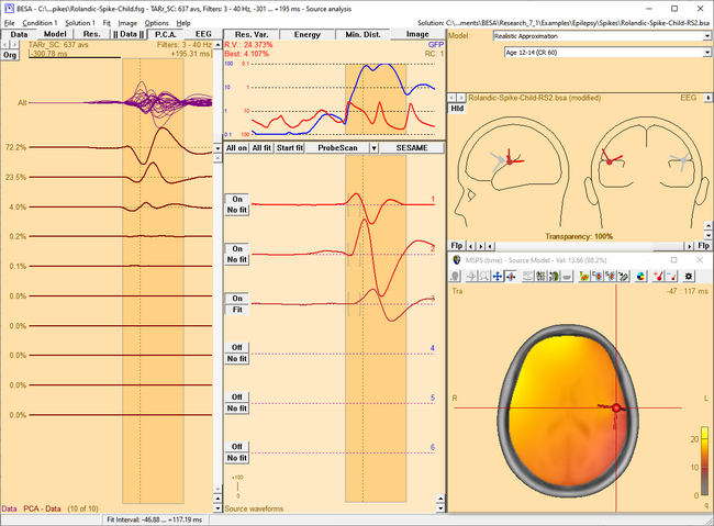 This figure shows the MSPS image applied on the three left-hemispheric sources in the solution 'Rolandic-Spike-Child-RS2.bsa'. The baseline is set from -300 ms to -50 ms. The right-hemispheric sources have been switched off. The fit interval is set to the latency range of large overall activity in the data (-43 ms : 117 ms). A realistic FEM model appropriate for the subject's age (12 years, conductivity ratios (cr) 50) is applied. The MSPS image does not show maxima at the modeled source locations and rather shows a spread q-value distribution.
 -
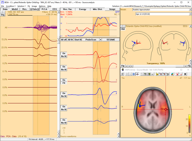 The MSPS image for the same latency range when the right-hemispheric sources have been included. The MSPS image appears more focal and shows maxima around the modeled brain regions. This indicates the substantial improvement of the solution by adding the right-hemispheric sources that model the propagation of the epileptic spike from the left to the right hemisphere (note the radiological side convention in the 3D window).
Time-Resolved MSPS
If the MSPS has been computed on time domain data, the image can be shown separately for each latency in the selected interval. After the MSPS has been computed for the marked epoch, double-click anywhere within this epoch to display the ratio of the probe source magnitude at the selected latency and the mean probe source magnitude in the baseline. Scanning the latency range by moving the cursor (e.g. with the left and right arrow cursor keys) provides a time-resolved MSPS image.
Time-resolved MSPS images are not available if the MSPS has been computed on data in the time-frequency domain.
Notes:
- You can hide or re-display the last computed image by selecting the corresponding entry in the Image menu.
- The current image can be exported to ASCII or BrainVoyager vmp-format from the Image menu.
- For scaling options, please refer to the scaling buttons popup menu .
- Parameters used for the MSPS calculations can be set in the General Settings tab of the Image Settings dialog box.
Source Sensitivity
Introduction
The 'Source sensitivity' function displays the sensitivity of the selected source in the current source model to activity in other brain regions. Sensitivity is defined as the fraction of power at the scanned brain location that is mapped onto the selected source.
To compute the source sensitivity, unit brain activity is modeled at different locations (probe source) throughout the brain. To this data, the current source model is applied to compute the source waveforms SCM of all modeled sources:
[math]\mathrm{S}_{\text{CM}} = \mathrm{L}_{\text{CM}}^{-1} \cdot \mathrm{L}_{\text{PS}}[/math]
Here LCM-1 is the regularized inverse operator for the current model, and LPS is the leadfield of the regional probe source (dimension [Nx3] for EEG and [Nx2] for MEG, respectively, where N is the number of sensors). The source amplitude SSS of the selected source in the model is a 3x3 (MEG: 2x2) sub-matrix of SCM (if the selected source is a regional source) or a 1x3-matrix (MEG: 1x2) (if the selected source is a dipole). The root mean square of the singular values of SCM is defined as the source sensitivity.
The 3D source sensitivity image displays this value for all locations on a grid specified under Image/Settings. Grid density can be specified in the Image Settings.
Applying the Source Sensitivity Image
The Source Sensitivity image is evoked from the Image menu or by pressing the corresponding hot key (default: V).
This function is enabled only when a solution with an active selected source is present in the Source Analysis window. The source sensitivity image then displays the sensitivity of the selected source to activity in other brain regions.
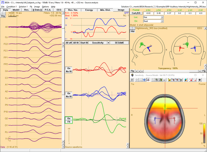
Notes:
- The sensitivity image is independent of the recorded sensor signals. It only depends on the current source model, the sensor configuration, the head model, and the regularization constant.
- If the regularization constant is set to zero, each source has a sensitivity of 100% to activity around its own location. With increasing regularization, the spatial filter becomes less focused, and the sensitivity of a source to activity at its location decreases.
- You can hide or re-display the last computed image by selecting the corresponding entry in the Image menu.
- The current image can be exported to ASCII or BrainVoyager vmp-format from the Image menu.
SESAME
This feature requires BESA Research 7.0 or higher.
SESAME (Sequential Semi-Analytic Monte-Carlo Estimation) is a Bayesian approach for estimating sources that uses Markov-Chain Monte-Carlo method for efficient computation of the probability distribution as described in Sommariva, S., & Sorrentino, A. "Sequential Monte Carlo samplers for semi-linear inverse problems and application to magnetoencephalography." Inverse Problems 30.11 (2014): 114020.
It allows to automatically estimate simultaneously the number of dipoles, their locations and time courses requiring virtually no user input. The algorithm is divided in two blocks:
- The first block consists of a Monte Carlo sampling algorithm that produces, with an adaptive number of iterations, a set of samples representing the posterior distribution for the number of dipoles and the dipole locations.
- The second block estimates the source time courses, given the number of dipoles and the dipole locations.
The Monte Carlo algorithm in the first block works by letting a set of weighted samples evolve with each iteration. At each iteration, the samples (a multi-dipole state) approximates the n-th element of a sequence of distributions p1, …, pN, that reaches the desired posterior distribution (pN = p(x|y)). The sequence is built as pN = p(x) p(y|x) α(n), such that α(1) = 0, α(N) = 1. The actual sequence of values of alpha is determined online. Dipole moments are estimated after the number of dipoles and the dipole locations have been estimated with the Monte Carlo procedure. This continues until a steady state is reached.
The SESAME image in BESA Research displays the final probability of source location along with an estimate for number of sources. Using the menu function Image / Export Image As... you have the option to save this SESAME image.
Non-uniform spatial priors for SESAME
By default, SESAME uses a uniform prior distribution on the source location. However, when the Weight by Image button at the top of the variance box is pressed and SESAME image is computed, the currently active 3D image will be used as non-uniform spatial priors for the SESAME computation (the positive values in the active 3D image, scaled to the current image maximum, are used as non-uniform spatial priors). The usage of non-uniform priors can effectively increase the source localization accuracy when the prior distribution is correct (A. Viani, G. Luria and A. Sorrentino, "Non-uniform spatial priors for multi-dipole localization from MEG/EEG data," 2022 IEEE International Conference on E-health Networking, Application & Services (HealthCom), Genoa, Italy, 2022, pp. 149-154, doi: 10.1109/HealthCom54947.2022.9982792). To use this method, a 3D image (e.g. source image or imported fMRI image) should be displayed in the 3D window. When the computation is finished, the Weight by Image button will be released.
Notes:
- Grid spacing: Due to memory and computational limitations, it is recommended to use SESAME with a grid spacing of 5 mm or more.
- Fit Interval: SESAME requires a fit interval of more than 2 samples to start the computation.
- Computation time: Computation speed during SESAME calculation depends on the grid spacing (computation is faster with larger grid spacing) and number of channels.
Brain Atlas
This feature requires BESA Research 7.0 or higher.
Introduction
Brain atlas is a priori data that can be applied over any discrete or distributed source image displayed in the 3D window. It is a reference value that strongly depends on the selected brain atlas and should not be used as medical reference since individual brains may differ from the brain atlas. The display settings can be adjusted in 3D Window Tab.
Brain Atlases
In BESA Research the atlases listed below are provided. BESA is not the author of the atlases; please cite the appropriate publications if you use any of the atlases in your publication.
Brainnetome
This is one of the most modern brain probabilistic atlas where structural, functional, and connectivity information was used to perform cortical parcellation. It was introduce by Fan and colleagues (2016), and is still work in progress. The atlas was created using data from 40 healthy adults taking part in the Human Connectome Project. In March 2018, the atlas consists of 246 structures labeled independently for each hemisphere. In BESA we provide the max probability map with labeling. Please visit the Brainnetome webpage to see more details related to the indicated brain regions (i.e. behavioral domains, paradigm classes and regions connectivity).
AAL
Automated Anatomical Labeling atlas was created in 2002 by Tzourio-Mazoyer and collegues (2002). It is the mostly used atlas nowadays. The atlas is based on the averaged brain of one subject (young male) who was scanned 27 times. The atlas resolution is 1 mm isometric. The brain sulci were drawn manually on every 2mm slice and then brain regions were automatically assigned. The atlas consists of 116 regions which are asymmetrical between hemispheres. The atlas is implemented as in the SPM12 toolbox.
Brodmann
The Brodmann map was created by Brodmann (1909). The brain regions were differentiated by cytoarchitecture of each cortical area using the Nissi method of cell staining. The digitalization of the original Brodmann map was performed by Damasio and Damasio (1989). The digitalized atlas consists of 44 fields that are symmetric between hemispheres. BESA used the atlas implementation as in Chris Roden’s MRICro software.
AAL2015
Automated Anatomical Labeling revision 2015. This is the updated AAL atlas. In comparison to the previous version (AAL) mainly the frontal lobe shows a higher degree of parcellation (Rolls, Joliot, and Tzourio-Mazoyer 2015). The atlas is implemented as in the SPM12 toolbox.
Talairach
Atlas was created in 1988 by Talairach and Tournoux (1988) and it is based on the post mortem brain slices of a 60 year old right handed European female. It was created by drawing and matching regions with the Brodmann map. The atlas is available at 5 tissue levels, however we used only the volumetric gyrus level as it is the most known in neuroscience and is the most appropriate for EEG. The atlas consists of 55 regions that are symmetric between hemispheres. The native resolution of the atlas was 0.43x0.43x2-5 mm. Please note that the poor resolution in Z direction is a direct consequence atlas definition, and since it is a post-mortem atlas it will not correctly match the brain template
(noticeable mainly on brain edges). The atlas digitalization was performed by Lancaster and colleagues (2000) resulting in a “golden standard” for neuroscience. The atlas was first implemented in a software called talairach daemon.
Yeo7 and Yeo17
Yeo7 and Yeo17 are the resting state functional connectivity atlases created by Yeo et al. (2011). For atlas creation 1000 subjects, coregistered using surface-based alignment were used. Two versions of parcellation were used resulting for the 7 and 17 networks (Yeo7 and Yeo17 atlas respectively). In the original publication atlases for two different levels of brain structure coverage were prepared: neocortex and liberal. In BESA products, only one of them (liberal) is available. Note that in comparison to the other atlases, here networks are reflected, rather than the individual brain structures. These atlases are in line with Resting State Source Montages.
Visualization modes
Just Labels
Displayed are crosshair coordinates (Talairach or MNI), the currently used brain atlas and the region name where the crosshair is placed. No atlas overlay will be visible on the 3D image.
brainCOLOR
All information is displayed as in “Just Labels” mode but also the atlas is visible as an overlay over the MRI. The coloring is performed using the algorithm introduced by Klein and colleagues (Klein et al. 2010). With this method of coloring the regions which are part of the same lobe are colored in a similar color but with different color shade. The shade is computed by the algorithm to make these regions visually differentiable from each other as much as possible.
Individual Color
In this mode the native brain atlas color is used if provided by the authors of the brain atlas (i.e. Yeo7). Where this was not available BESA autogenerated colors for the atlas using an approach similar to political map coloring. This approach aims to differentiate most regions that are adjacent to each other and no presumptions on lobes is applied.
Contour
Only region contours (borders between atlas regions) are drawn with blue color. This is the default mode in BESA Research.
References
- Brodmann, Korbinian. 1909. Vergleichende Lokalisationslehre Der Großhirnrinde. Leipzig: Barth. https://www.livivo.de/doc/437605.
- Damasio, Hanna, and Antonio R. Damasio. 1989. Lesion Analysis in Neuropsychology. Oxford University Press, USA.
- Fan, Lingzhong, Hai Li, Junjie Zhuo, Yu Zhang, Jiaojian Wang, Liangfu Chen, Zhengyi Yang, et al. 2016. “The Human Brainnetome Atlas: A New Brain Atlas Based on Connectional Architecture.” Cerebral Cortex 26 (8): 3508–26. https://doi.org/10.1093/cercor/bhw157.
- Klein, Arno, Andrew Worth, Jason Tourville, Bennett Landman, Tito Dal Canton, Satrajit S. Ghosh, and David Shattuck. 2010. “An Interactive Tool for Constructing Optimal Brain Colormaps.” https://mindboggle.info/braincolor/colormaps/index.html.
- Lancaster, Jack L., Marty G. Woldorff, Lawrence M. Parsons, Mario Liotti, Catarina S. Freitas, Lacy Rainey, Peter V. Kochunov, Dan Nickerson, Shawn A. Mikiten, and Peter T. Fox. 2000. “Automated Talairach Atlas Labels for Functional Brain Mapping.” Human Brain Mapping 10 (3): 120–131.
- Rolls, Edmund T., Marc Joliot, and Nathalie Tzourio-Mazoyer. 2015. “Implementation of a New Parcellation of the Orbitofrontal Cortex in the Automated Anatomical Labeling Atlas.” NeuroImage 122 (November): 1–5. https://doi.org/10.1016/j.neuroimage.2015.07.075.
- Talairach, J, and P Tournoux. 1988. Co-Planar Stereotaxic Atlas of the Human Brain. 3-Dimensional Proportional System: An Approach to Cerebral Imaging. Thieme.
- Thomas Yeo, B. T., F. M. Krienen, J. Sepulcre, M. R. Sabuncu, D. Lashkari, M. Hollinshead, J. L. Roffman, et al. 2011. “The Organization of the Human Cerebral Cortex Estimated by Intrinsic Functional Connectivity.” Journal of Neurophysiology 106 (3): 1125–65. https://doi.org/10.1152/jn.00338.2011.
- Tzourio-Mazoyer, N., B. Landeau, D. Papathanassiou, F. Crivello, O. Etard, N. Delcroix, B. Mazoyer, and M. Joliot. 2002. “Automated Anatomical Labeling of Activations in SPM Using a Macroscopic Anatomical Parcellation of the MNI MRI Single-Subject Brain.” NeuroImage 15 (1): 273–89. https://doi.org/10.1006/nimg.2001.0978.
Slice View
This feature requires BESA Research 7.1 or higher.
A convenient way to review MRI data and export it in graphical form is a multi-slice view. To enable multi-slice view press the toggle multiple view button until the slice view is shown in the 3D window.
In this view discrete sources, distributed sources and brain atlas can be also be overlayed. The display matrix can be adjusted by slice view controls that are available in the 3D Window tab of the Preferences Dialog Box. One of the following slicing direction can be selected: Transverse, Coronal, Sagittal by pressing the appropriate button in the 3D window toolbar.
By adjusting First slice and Last slice sliders, the span of the volume that will be displayed can be adjusted. The interval between slices can be adjusted by changing the Spacing slider value. The layout of slices will be automatically adjusted to fill the full space of the main window. All values in the sliders are given in mm.
Note: The last slice value will be adjusted to the closest possible number matching the given first slice and spacing value. During multi-slice view the cursor is disabled and no atlas information is provided.
Glassbrain
This feature requires BESA Research 7.1 or higher.
The glass brain can be enabled or disabled in one of the following ways:
- by pressing the button
 in the toolbar,
- by using the shortcut SHIFT-G or
- by checking the checkbox in Preferences, 3D Display tab.
The transparency value of the glass brain can be adjusted in one of the following ways:
- by a slider/edit box in Preferences, 3D Display tab or
- by using the keyboard shortcut SHIFT-UP (to increase transparency by 10%) or SHIFT-DOWN (to decrease transparency by 10%).
Note that If a distributed solution is displayed together with the glass brain, a notification is displayed in the left bottom corner of 3D window to prevent misconception of the glass brain as a cortical image:
“Volume-based image only", which means that the results of distributed source analysis images are visualized only for the current MRI slice, and are not projected to the displayed surface.
| Review | |
|---|---|
| Source Analysis |
|
| Integration with MRI and fMRI | |
| Source Coherence | |
| Export | |
| MATLAB Interface | |
| Special Topics | |
