Difference between revisions of "How to Prepare Data for BESA Connectivity"
(→Examples) |
(→Export data using Matlab) |
||
| (19 intermediate revisions by 2 users not shown) | |||
| Line 1: | Line 1: | ||
{{BESAInfobox | {{BESAInfobox | ||
|title = Module information | |title = Module information | ||
| − | |module = BESA Research Basic or higher | + | |module = BESA Research Basic or higher<br/>BESA Connectivity |
| − | BESA Connectivity | + | |version = BESA Research 7.0 or higher<br/>BESA Connectivity 1.0 or higher |
| − | |version = 7.0 or higher | + | |
}} | }} | ||
| Line 12: | Line 11: | ||
# A file containing the binary data matrix. All epochs in the data file need to have the same length, the same stimulus position, the same baseline interval, and the same channel configuration. | # A file containing the binary data matrix. All epochs in the data file need to have the same length, the same stimulus position, the same baseline interval, and the same channel configuration. | ||
# A header file in ASCII format. | # A header file in ASCII format. | ||
| − | # A channel description file in ASCII format. Two types of files are supported: elp files and bsa files. | + | # A channel description file in ASCII format. Two types of files are supported: [[#ELP file format|elp]] files and [[BSA file format|bsa]] files. |
== File format descriptions == | == File format descriptions == | ||
| Line 33: | Line 32: | ||
| nChannels= | | nChannels= | ||
| [1 ... 1024] | | [1 ... 1024] | ||
| − | | Number of channels | + | | Number of channels. |
|- | |- | ||
| 3 | | 3 | ||
| sRate= | | sRate= | ||
| [0.0001 ... ] | | [0.0001 ... ] | ||
| − | | Sampling rate in Hz | + | | Sampling rate (samples/second) in Hz. |
|- | |- | ||
| 4 | | 4 | ||
| nSamples= | | nSamples= | ||
| [1 ...] | | [1 ...] | ||
| − | | Total number of samples in file | + | | Total number of samples in file. |
|- | |- | ||
| 5 | | 5 | ||
| format= | | format= | ||
| float | | float | ||
| − | | Format of the data in the binary file | + | | Format of the data in the binary file. |
|- | |- | ||
| 6 | | 6 | ||
| file= | | file= | ||
| − | | Name of binary file | + | | Name of binary file. |
| − | | Name of binary file | + | | Name of binary file without path information. |
|- | |- | ||
| 7 | | 7 | ||
| prestimulus= | | prestimulus= | ||
| − | | 500.000 | + | | 500.000 |
| Pre-stimulus interval in milliseconds. If negative, then the epoch starts after the stimulus. This effectively means that the value of prestimulus denotes the position of the stimulus in the epoch (milliseconds after epoch start). | | Pre-stimulus interval in milliseconds. If negative, then the epoch starts after the stimulus. This effectively means that the value of prestimulus denotes the position of the stimulus in the epoch (milliseconds after epoch start). | ||
|- | |- | ||
| Line 63: | Line 62: | ||
| epochs= | | epochs= | ||
| | | | ||
| − | | Number of epochs in the data file | + | | Number of epochs in the data file. |
|- | |- | ||
| 9 | | 9 | ||
| baselineStart= | | baselineStart= | ||
| | | | ||
| − | | Baseline start relative to the stimulus position. | + | | Baseline start relative to the stimulus position. The value should be given in milliseconds. |
|- | |- | ||
| 10 | | 10 | ||
| baselineEnd= | | baselineEnd= | ||
| | | | ||
| − | | Baseline end relative to the stimulus position. Must be >= baselineStart | + | | Baseline end relative to the stimulus position. Must be >= baselineStart. The value should be given in milliseconds. |
|- | |- | ||
| 11 | | 11 | ||
| Line 79: | Line 78: | ||
| | | | ||
| Epoch length in milliseconds. This parameter is optional and can be added for convenience. If not given, the epoch length is calculated from the overall number of samples, the sampling rate, and the number of epochs. | | Epoch length in milliseconds. This parameter is optional and can be added for convenience. If not given, the epoch length is calculated from the overall number of samples, the sampling rate, and the number of epochs. | ||
| + | |- | ||
| + | | 11 | ||
| + | | Padding= | ||
| + | | 2000.000 | ||
| + | | Information concerning extra data values that surround the epoch to provide padding for wavelets, expressed in milliseconds. If exported from BESA Research the default value is 2000ms. | ||
|- | |- | ||
| 12 | | 12 | ||
| Line 189: | Line 193: | ||
| RGB color value | | RGB color value | ||
|} | |} | ||
| + | |||
| + | The coordinate system is defined by a sphere with unit dimensions, which is fitted to the coordinates of sensors on the head. In the absence of [[Integration with MRI and fMRI|co-registration]] information with individual MRI data, the axes are defined by reference points on the head known as fiducials. The reference points are normally the nasion (NAS), the left preauricular point (LPA), and the right preauricular point (RPA). The direction of the x axis is defined by the line joining LPA and RPA, positive towards RPA. The direction of the y axis is defined by the line through NAS that is perpendicular to the x axis (positive towards NAS). The z axis is perpendicular to the x and y axes, and goes up out of the upper part of the head (e.g. Cz). On average, the center of the unit sphere is about 4 cm above the origin of the head coordinate system. | ||
=== Binary data matrix file format === | === Binary data matrix file format === | ||
| + | |||
| + | The binary data matrix is saved in float format and contains ''<Number of epochs> * <Number of samples per epoch> * <Number of channels>'' values. These are stored in the following order: | ||
| + | *Slowest index: epochs | ||
| + | *Next index: samples | ||
| + | *Fastest index: channels | ||
| + | This is the so-called multiplexed file format. The default extension for this header file is: ''*.dat'' | ||
== Export data using BESA Research == | == Export data using BESA Research == | ||
| + | Please follow the steps in the BESA Research 7.1 tutorial, chapter 12 - Time-frequency Analysis, Connectivity Analysis and Beamforming: [https://www.besa.de/wp-content/uploads/2021/04/BESA-Research-7.1-Tutorial.pdf Link] | ||
| + | |||
| + | == Batch export data using BESA Research == | ||
| + | ''(requires BESA Researh version 7.1)'' | ||
| + | |||
| + | BESA Research provides batch processing multiple files to export data for BESA Connectivity. This will simplify and speed up your analysis if you need to apply the same data preparation steps for a large number of files. | ||
| + | |||
| + | This section will provide the batch that is required to export the data epochs and will also explain additional steps that need to be performed to load the exported data sets into BESA Connectivity. | ||
| + | |||
| + | ==== BESA Research Batch ==== | ||
| + | |||
| + | The batch commands required to export all epochs around trigger #1 is displayed below. The first step is to set the specific montage in which all epochs should be exported. Then, the default epoch length needs to be set. In this example, epochs range from -500ms to 2000ms. However, preceding and succeeding padding intervals of 2000ms are required to avoid edge effects during time-frequency transformation. Therefore, the resulting default epoch is set to -2500ms to 4000ms. After this, trigger #1 is selected and epochs are exported to ''C:\Users\<USERNAME>\Documents\BESA\Research_7_1\Export\Batch Export\''. Finally, the batch will also export the channel configuration file (*.elp) in case of sensor data. In case of source data, the corresponding source configuration file (*.bsa) that was used to create the respective source montage needs to be copied to the output folder manually! | ||
| + | |||
| + | Please note: adjust the ''<USERNAME>'' placeholder or the export path according to your needs. | ||
| + | |||
| + | <source lang="dos"> | ||
| + | ; Set montage | ||
| + | MAINMontage(DMN with Noise Sources, Wait if invalid, GlobalMontage) | ||
| + | ; Set epoch length. Note: add 2000ms padding ad start & end | ||
| + | EditDefaultEpoch(-2500.000,4000.000) | ||
| + | ; | ||
| + | ; Export epochs for trigger #1 | ||
| + | TriggerSelect(1) | ||
| + | MAINExport(%basename%-export-T1, C:\Users\<USERNAME>\Documents\BESA\Research_7_1\Export\Batch Export\, Epochs, SimpleBin, Current, FiltOff, NoResample, Replace, -, , WholeFile) | ||
| + | ; | ||
| + | ; Export channel configuration file | ||
| + | MAINMarkBlock(Rawdata,-,1) | ||
| + | MAINExport(%basename%-export-T1, C:\Users\<USERNAME>\Documents\BESA\Research_7_1\Export\Batch Export\, Segment, ASCmul, Original, FiltOff, NoResample, Replace, -, , WholeFile) | ||
| + | </source > | ||
| + | |||
| + | This batch can be downloaded from the following link and loaded in the ''Batch'' tab of the ''Batch Processing'' module:[[Media:Batch_Export_for_BESA_Connectivity.bbat|Download link.]] | ||
| + | |||
| + | ==== Additional Steps ==== | ||
| + | |||
| + | In order to be able to import the saved data sets into BESA Connectivity, there are a few changes that need to be made to the exported *.generic file(s). | ||
| + | |||
| + | When opening the *.generic file with a text editor you will realize that the format slightly differs from the file format description above. the following images compare the exported file (left) and the adjusted file that can be imported into BESA Connectivity (right). | ||
| + | |||
| + | <!-- | ||
| + | --><p>[[File:Generic_File_Unchanged.png|150px|top]][[File:Generic File Modified.png|150px|alt text]]</p> | ||
| + | |||
| + | |||
| + | Please adjust or add the following sections to the *.generic file: | ||
| + | * File format version: set to V1.1 | ||
| + | * Add lines for baselineStart, baselineEnd and epochLength. Note: the time stamps do not include the padding intervals! | ||
| + | * Add the line to specify the padding interval of 2000ms. | ||
| + | * Add the specification of the condition name. | ||
| + | * Add one line per channel/source and specify the its label and unit. | ||
| + | |||
| + | Save the file after performing the changes. | ||
| + | |||
| + | If you are working with source data, make sure that the corresponding source configuration file (*.bsa) has the same basename as the *.generic file. Otherwise, BESA Connectivity will not be able to load the file. | ||
| + | |||
| + | Now the exported data sets are ready to be loaded into BESA Connectivity! | ||
== Export data using Matlab == | == Export data using Matlab == | ||
| + | |||
| + | We provide several Matlab routines for exporting the required data files from Matlab to BESA Connectivity. The scripts can be downloaded from the following website: [http://www.besa.de/downloads/matlab/ MATLAB Scripts]. | ||
| + | |||
| + | The <code>Matlab_to_BESAConnectivity.m</code> script (download available here: [https://github.com/BESA-GmbH/BESA-MATLAB-Scripts/releases/latest/download/BesaConnectivityScripts.zip BESA Connectivity Scripts]) can be used as an example to generate and export data from MATLAB to BESA Connectivity. | ||
| + | It shows how to define required parameters, generates example sine waves and calls the export function <code>besa_save2Connectivity</code> (included in: [https://github.com/BESA-GmbH/BESA-MATLAB-Scripts/releases/latest/download/MATLAB2BESA.zip MATLAB2BESA]) to store the simulated example data to disc. It will store the file containing the binary data matrix, as well as the header file and channel description file in ASCII format. | ||
| + | |||
| + | The script can be easily adopted to export your trial data do BESA Connectivity for time-frequency and connectivity analysis! | ||
== Examples == | == Examples == | ||
| Line 201: | Line 274: | ||
Minimal examples for data files that can be imported in BESA Connectivity can be downloaded here. | Minimal examples for data files that can be imported in BESA Connectivity can be downloaded here. | ||
# EEG data: this data set contains 25 trials (trial length: -400ms to 1200ms) of scalp data with 27 electrodes at a sampling rate of 320 samples/second.<!-- | # EEG data: this data set contains 25 trials (trial length: -400ms to 1200ms) of scalp data with 27 electrodes at a sampling rate of 320 samples/second.<!-- | ||
| − | --><p>Download link.</p><!-- | + | --><p>[[Media:BESA_Connectivity_EEG_data.zip|Download link.]]</p><!-- |
--><p>[[File:BESA_Connectivity_Set_Parameters_EEG_Data.png|400px]][[File:BESA_Connectivity_Run_Analysis_EEG_Data_iCoh.png|400px|alt text]]</p> | --><p>[[File:BESA_Connectivity_Set_Parameters_EEG_Data.png|400px]][[File:BESA_Connectivity_Run_Analysis_EEG_Data_iCoh.png|400px|alt text]]</p> | ||
# Source data: this data set contains 33 trials (trial length: -400ms to 1200ms) of source data with 19 dipoles at a sampling rate of 320 samples/second.<!-- | # Source data: this data set contains 33 trials (trial length: -400ms to 1200ms) of source data with 19 dipoles at a sampling rate of 320 samples/second.<!-- | ||
| − | --><p>Download link.</p><!-- | + | --><p>[[Media:BESA_Connectivity_Source_data.zip|Download link.]]</p><!-- |
--><p>[[File:BESA_Connectivity_Set_Parameters_Source_Data.png|400px]][[File:BESA_Connectivity_Run_Analysis_Source_Data_iCoh.png|400px|alt text]]</p> | --><p>[[File:BESA_Connectivity_Set_Parameters_Source_Data.png|400px]][[File:BESA_Connectivity_Run_Analysis_Source_Data_iCoh.png|400px|alt text]]</p> | ||
| − | [[Category:Connectivity]] [[Category:Time-Frequency]] | + | |
| + | [[Category:Connectivity]] [[Category:Time-Frequency]] [[Category:Data Import/Export]] | ||
Latest revision as of 13:03, 27 August 2021
| Module information | |
| Modules | BESA Research Basic or higher BESA Connectivity |
| Version | BESA Research 7.0 or higher BESA Connectivity 1.0 or higher |
Contents
Note and general remarks
This article applies to data that are prepared using BESA Research. It is also possible to read data prepared by other programs. For the requirements, please refer to the BESA Connectivity manual, the chapter on "Loading data that were created in other software" and the chapter "File formats".
BESA Connectivity needs the following data:
- A file containing the binary data matrix. All epochs in the data file need to have the same length, the same stimulus position, the same baseline interval, and the same channel configuration.
- A header file in ASCII format.
- A channel description file in ASCII format. Two types of files are supported: elp files and bsa files.
File format descriptions
Header file format
The header file is a standard ASCII file. It contains the following lines:
| Line | Entry | Possible values | Description |
|---|---|---|---|
| 1 | BESA Generic Data v1.1 | File format version | |
| 2 | nChannels= | [1 ... 1024] | Number of channels. |
| 3 | sRate= | [0.0001 ... ] | Sampling rate (samples/second) in Hz. |
| 4 | nSamples= | [1 ...] | Total number of samples in file. |
| 5 | format= | float | Format of the data in the binary file. |
| 6 | file= | Name of binary file. | Name of binary file without path information. |
| 7 | prestimulus= | 500.000 | Pre-stimulus interval in milliseconds. If negative, then the epoch starts after the stimulus. This effectively means that the value of prestimulus denotes the position of the stimulus in the epoch (milliseconds after epoch start). |
| 8 | epochs= | Number of epochs in the data file. | |
| 9 | baselineStart= | Baseline start relative to the stimulus position. The value should be given in milliseconds. | |
| 10 | baselineEnd= | Baseline end relative to the stimulus position. Must be >= baselineStart. The value should be given in milliseconds. | |
| 11 | epochLength= | Epoch length in milliseconds. This parameter is optional and can be added for convenience. If not given, the epoch length is calculated from the overall number of samples, the sampling rate, and the number of epochs. | |
| 11 | Padding= | 2000.000 | Information concerning extra data values that surround the epoch to provide padding for wavelets, expressed in milliseconds. If exported from BESA Research the default value is 2000ms. |
| 12 | conditionName= | Name of the condition that identifies it. | |
| 13 | channelUnits= | Unit that the data are stored in the binary file. For EEG data, it should be one of µV, mV, V, µV/cm². For source data, it should be one of nAm, nAm/cm², nAm/cm³. For MEG data, it should be one of fT, pT, fT/cm, pT/cm, µV/cm².
This entry is repeated <nChannels> times. |
Channel configuration file format
The channel description file is an ASCII file. Two types of files are supported: .elp files and .bsa files.
ELP file format
Elp files describe surface channel coordinates using spherical coordinates (theta, phi). It contains one line for each channel in the data file. Each line contains the following entries:
| Column | Entry | Possible values | Description |
|---|---|---|---|
| 1 | Channel type | EEG (scalp electrode) SCP (scalp electrode) |
This column denotes the type of the channel. |
| 2 | Channel label | Fpz Fz |
Channel label. Is not allowed to contain blanks. |
| 3 | Azimuth (theta) | [-180.00 ... 180.00] | Spherical azimuth angle in degrees (optional entry). |
| 4 | Latitude (phi) | [-90.00 ... 90.00] | Spherical latitude angle in degrees (optional entry). |
BSA file format
Bsa files describe source channel data. They have a header section for format version and readability, followed by one line for each source channel.
| Column | Entry | Possible values | Description |
|---|---|---|---|
| 1 | Channel type | RegSrc (regional source)
DipSrc (dipole) |
This column denotes the type of the channel. |
| 2 | x location | x coordinate of the channel. | |
| 3 | y location | y coordinate of the channel. | |
| 4 | z location | z coordinate of the channel. | |
| 5 | x orientation | x orientation of the channel. | |
| 6 | y orientation | y orientation of the channel. | |
| 7 | z orientation | z orientation of the channel. | |
| 8 | Color | [0 … 255*255*255] | RGB color value |
The coordinate system is defined by a sphere with unit dimensions, which is fitted to the coordinates of sensors on the head. In the absence of co-registration information with individual MRI data, the axes are defined by reference points on the head known as fiducials. The reference points are normally the nasion (NAS), the left preauricular point (LPA), and the right preauricular point (RPA). The direction of the x axis is defined by the line joining LPA and RPA, positive towards RPA. The direction of the y axis is defined by the line through NAS that is perpendicular to the x axis (positive towards NAS). The z axis is perpendicular to the x and y axes, and goes up out of the upper part of the head (e.g. Cz). On average, the center of the unit sphere is about 4 cm above the origin of the head coordinate system.
Binary data matrix file format
The binary data matrix is saved in float format and contains <Number of epochs> * <Number of samples per epoch> * <Number of channels> values. These are stored in the following order:
- Slowest index: epochs
- Next index: samples
- Fastest index: channels
This is the so-called multiplexed file format. The default extension for this header file is: *.dat
Export data using BESA Research
Please follow the steps in the BESA Research 7.1 tutorial, chapter 12 - Time-frequency Analysis, Connectivity Analysis and Beamforming: Link
Batch export data using BESA Research
(requires BESA Researh version 7.1)
BESA Research provides batch processing multiple files to export data for BESA Connectivity. This will simplify and speed up your analysis if you need to apply the same data preparation steps for a large number of files.
This section will provide the batch that is required to export the data epochs and will also explain additional steps that need to be performed to load the exported data sets into BESA Connectivity.
BESA Research Batch
The batch commands required to export all epochs around trigger #1 is displayed below. The first step is to set the specific montage in which all epochs should be exported. Then, the default epoch length needs to be set. In this example, epochs range from -500ms to 2000ms. However, preceding and succeeding padding intervals of 2000ms are required to avoid edge effects during time-frequency transformation. Therefore, the resulting default epoch is set to -2500ms to 4000ms. After this, trigger #1 is selected and epochs are exported to C:\Users\<USERNAME>\Documents\BESA\Research_7_1\Export\Batch Export\. Finally, the batch will also export the channel configuration file (*.elp) in case of sensor data. In case of source data, the corresponding source configuration file (*.bsa) that was used to create the respective source montage needs to be copied to the output folder manually!
Please note: adjust the <USERNAME> placeholder or the export path according to your needs.
; Set montage
MAINMontage(DMN with Noise Sources, Wait if invalid, GlobalMontage)
; Set epoch length. Note: add 2000ms padding ad start & end
EditDefaultEpoch(-2500.000,4000.000)
;
; Export epochs for trigger #1
TriggerSelect(1)
MAINExport(%basename%-export-T1, C:\Users\<USERNAME>\Documents\BESA\Research_7_1\Export\Batch Export\, Epochs, SimpleBin, Current, FiltOff, NoResample, Replace, -, , WholeFile)
;
; Export channel configuration file
MAINMarkBlock(Rawdata,-,1)
MAINExport(%basename%-export-T1, C:\Users\<USERNAME>\Documents\BESA\Research_7_1\Export\Batch Export\, Segment, ASCmul, Original, FiltOff, NoResample, Replace, -, , WholeFile)
This batch can be downloaded from the following link and loaded in the Batch tab of the Batch Processing module:Download link.
Additional Steps
In order to be able to import the saved data sets into BESA Connectivity, there are a few changes that need to be made to the exported *.generic file(s).
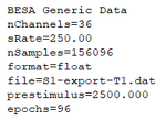
When opening the *.generic file with a text editor you will realize that the format slightly differs from the file format description above. the following images compare the exported file (left) and the adjusted file that can be imported into BESA Connectivity (right).
Please adjust or add the following sections to the *.generic file:
- File format version: set to V1.1
- Add lines for baselineStart, baselineEnd and epochLength. Note: the time stamps do not include the padding intervals!
- Add the line to specify the padding interval of 2000ms.
- Add the specification of the condition name.
- Add one line per channel/source and specify the its label and unit.
Save the file after performing the changes.
If you are working with source data, make sure that the corresponding source configuration file (*.bsa) has the same basename as the *.generic file. Otherwise, BESA Connectivity will not be able to load the file.
Now the exported data sets are ready to be loaded into BESA Connectivity!
Export data using Matlab
We provide several Matlab routines for exporting the required data files from Matlab to BESA Connectivity. The scripts can be downloaded from the following website: MATLAB Scripts.
The Matlab_to_BESAConnectivity.m script (download available here: BESA Connectivity Scripts) can be used as an example to generate and export data from MATLAB to BESA Connectivity.
It shows how to define required parameters, generates example sine waves and calls the export function besa_save2Connectivity (included in: MATLAB2BESA) to store the simulated example data to disc. It will store the file containing the binary data matrix, as well as the header file and channel description file in ASCII format.
The script can be easily adopted to export your trial data do BESA Connectivity for time-frequency and connectivity analysis!
Examples
Minimal examples for data files that can be imported in BESA Connectivity can be downloaded here.
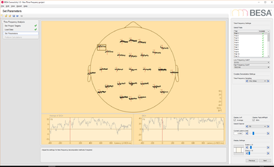
- EEG data: this data set contains 25 trials (trial length: -400ms to 1200ms) of scalp data with 27 electrodes at a sampling rate of 320 samples/second.
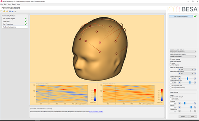
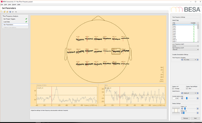
- Source data: this data set contains 33 trials (trial length: -400ms to 1200ms) of source data with 19 dipoles at a sampling rate of 320 samples/second.
