Difference between revisions of "BESA Research Batch Processing"
| Line 242: | Line 242: | ||
|- | |- | ||
|style="text-align:center;" width="10%"|'''%basename%''' | |style="text-align:center;" width="10%"|'''%basename%''' | ||
| − | |width="40%"|replaced by the basename of the | + | |width="40%"|replaced by the basename of the currently opened file. |
|width="40%"|If the data file is named "<span style="color:#ff9c00;">f-spike.fsg</span>", "<span style="color:#ff9c00;">%basename%-export.fsg</span>" will be interpreted as "<span style="color:#ff9c00;">f-spike-export.fsg</span>". | |width="40%"|If the data file is named "<span style="color:#ff9c00;">f-spike.fsg</span>", "<span style="color:#ff9c00;">%basename%-export.fsg</span>" will be interpreted as "<span style="color:#ff9c00;">f-spike-export.fsg</span>". | ||
|- | |- | ||
|style="text-align:center;"|'''%basename-n%''' | |style="text-align:center;"|'''%basename-n%''' | ||
| − | |replaced by the basename of the | + | |replaced by the basename of the currently opened file, but removing the last "n" characters from the name. |
|If the data file is named "<span style="color:#ff9c00;">dongle-BB.fsg</span>", "<span style="color:#ff9c00;">%basename-3%</span>" will be replaced by "<span style="color:#ff9c00;">dongle</span>", because the last 3 characters of the basename have been removed. | |If the data file is named "<span style="color:#ff9c00;">dongle-BB.fsg</span>", "<span style="color:#ff9c00;">%basename-3%</span>" will be replaced by "<span style="color:#ff9c00;">dongle</span>", because the last 3 characters of the basename have been removed. | ||
|- | |- | ||
|style="text-align:center;"|'''%-nbasename%''' | |style="text-align:center;"|'''%-nbasename%''' | ||
| − | |replaced by the basename of the | + | |replaced by the basename of the currently opened file, but removing the first "n" characters from the name. |
|If the data file is named "<span style="color:#ff9c00;">BB-dongle.fsg</span>", "<span style="color:#ff9c00;">%-3basename%</span>" will be replaced by "<span style="color:#ff9c00;">dongle</span>", because the first 3 characters of the basename have been removed. | |If the data file is named "<span style="color:#ff9c00;">BB-dongle.fsg</span>", "<span style="color:#ff9c00;">%-3basename%</span>" will be replaced by "<span style="color:#ff9c00;">dongle</span>", because the first 3 characters of the basename have been removed. | ||
| + | |- | ||
| + | |style="text-align:center;"|<span title="Requires BESA Research 7.1 or higher"><u>'''%orgbasename%'''</u></span> | ||
| + | |replace by basename of the current file in the file list (it has the same meaning as %basename% if no MAINFileOpen batch command was used in command list) | ||
| + | | | ||
| + | |- | ||
| + | |style="text-align:center;"|<span title="Requires BESA Research 7.1 or higher"><u>'''%base%'''</u></span> | ||
| + | |replace by basename of the current file without the path | ||
| + | | | ||
| + | |- | ||
| + | |style="text-align:center;"|<span title="Requires BESA Research 7.1 or higher"><u>'''%orgbase%'''</u></span> | ||
| + | |replace by basename of the current file in the file list without the path | ||
| + | |- | ||
| + | |style="text-align:center;"|<span title="Requires BESA Research 7.1 or higher"><u>'''%ext%'''</u></span> | ||
| + | |replace by extension of the current file | ||
| + | | | ||
| + | |- | ||
| + | |style="text-align:center;"|<span title="Requires BESA Research 7.1 or higher"><u>'''%orgext%'''</u></span> | ||
| + | |replace by extension of the current file in the file list | ||
| + | | | ||
| + | |- | ||
| + | |style="text-align:center;"|<span title="Requires BESA Research 7.1 or higher"><u>'''%basefolder%'''</u></span> | ||
| + | |replace by folder of the current file | ||
| + | | | ||
| + | |- | ||
| + | |style="text-align:center;"|<span title="Requires BESA Research 7.1 or higher"><u>'''%orgbasefolder%'''</u></span> | ||
| + | |replace by folder of the current file in the file list | ||
| + | | | ||
| + | |- | ||
| + | |style="text-align:center;"|<span title="Requires BESA Research 7.0 or higher"><u>'''%t%'''</u></span> | ||
| + | |Log batch command only: time since start of batch on current file | ||
| + | | | ||
| + | |- | ||
| + | |style="text-align:center;"|<span title="Requires BESA Research 7.0 or higher"><u>'''%T%'''</u></span> | ||
| + | |Log batch command only: current date and time | ||
| + | | | ||
| + | |- | ||
| + | |style="text-align:center;"|<span title="Requires BESA Research 7.0 or higher"><u>'''%label%'''</u></span> | ||
| + | |Replace label of the most recent marked block by the block label, not including no. of averages | ||
| + | | | ||
| + | |- | ||
| + | |style="text-align:center;"|<span title="Requires BESA Research 7.0 or higher"><u>'''%LABEL%'''</u></span> | ||
| + | | Replace label of the most recent marked block by the block label, including no. of averages | ||
| + | |||
| + | | | ||
|- | |- | ||
|style="text-align:center;"|'''%scripts%''' | |style="text-align:center;"|'''%scripts%''' | ||
Revision as of 14:41, 4 May 2021
| Module information | |
| Modules | BESA Research Basic or higher |
| Version | 6.1 or higher |
Contents
- 1 Combine Conditions and Batch Module: Introduction
- 2 File List Tab
- 3 Batch Processing
- 4 Combine Conditions, Channels
- 4.1 Combine Condition Scripts
- 4.2 Condition List Tab
- 4.3 Channel List Tab
- 4.4 Run Scripts Tab
- 4.5 How to Create Grand Averages
- 4.6 How to Generate Differences Between Conditions
- 4.7 How to Merge Files
- 4.8 How to Remove Unwanted Averages
- 4.9 How to Rename Conditions
- 4.10 How to Change the Sampling Rate
- 4.11 Example: Create grand average and combinations of conditions
- 4.12 Example: Average files from different experiments
Combine Conditions and Batch Module: Introduction
Functions of this module are started by selecting the menu operations "ERP / Combine Conditions..." and "Process / Batch Scripts...".
- Combine Condition Scripts provides various operations on BESA averages.
- Batch Scripts provides batch operations on all data files.
- Note that a batch script can also be performed on the current file by selecting "Process / Run Batch..." or by typing the shortcut key "R".
File List Tab
Define a list of files on which the operations will be performed. The tab is the same for Combine Conditions Scripts and for Batch Scripts. Combine Conditions Scripts only allows you to open BESA average files (e.g. *.fsg and *.avr, but also .mul, .raw, .swf, and .foc if the files have a defined pre-stimulus interval), whereas Batch Scripts allows you to open any data file whose format is known to BESA Research.
When the Combine-Conditions or the Batch module is started, all currently opened (Combine-Conditions: averages only) files are displayed in the list.
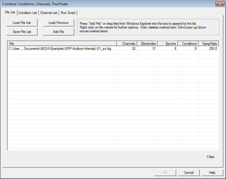
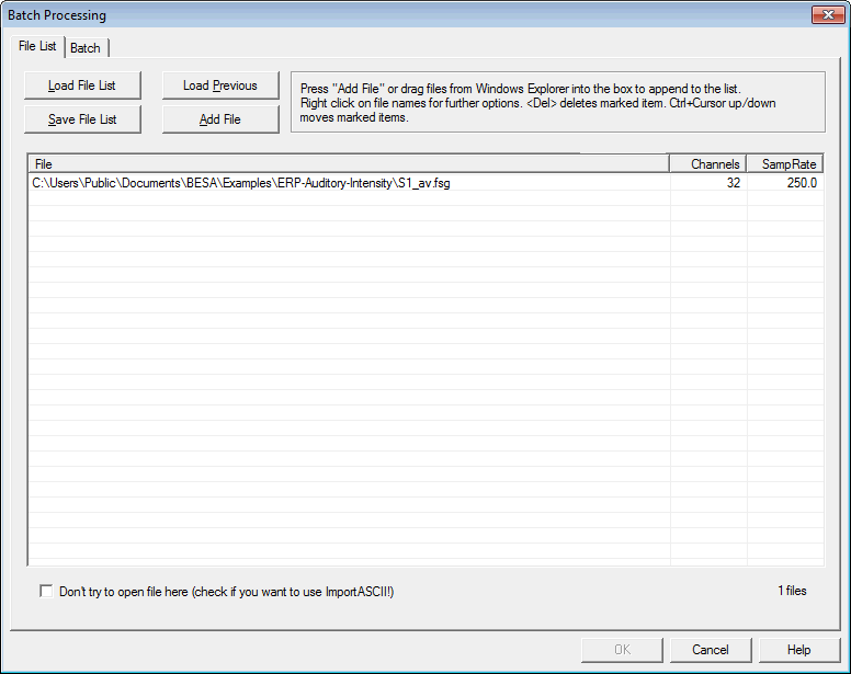
To the right of each file name, the number of electrodes, total number of channels, and the sampling rate used in the file are displayed. In the Combine-Conditions module, the number of Epochs (segments) and the number of differently-named conditions are also shown.
Add files to the list
- Press the Add File button.
- Drag one or more files from Windows Explorer onto the window.
Remove files from the list
- Right click on the file name and confirm the delete operation in the resulting dialog.
- Mark one or more file names in the list (e.g. hold down the Ctrl key to mark multiple files). Right click to obtain the context menu and select "Delete", or just press the Del key.
Reorder files within the current file list
- Right click on the file name and select "Move Up" or "Move Down".
- Mark one or more file names in the list (e.g. hold down the Ctrl key to mark multiple files). Right click to obtain the context menu and select "Move Up" or "Move Down", or hold down the Ctrl key and press the Up and Down arrows.
Sort the current file list alphabetically
- Click on the File bar above the list
Save the current file list
- Press the Save File List button.
Load a file list
- Press the Load File List button, or the Load Previous button to load the most recently used file list.
Which conditions are read from a source file? (Combine-Conditions module only)
- Normally, all conditions are read from a source file. To exclude one or more segments from operations in the Combine Conditions module, mark the segments as artifacts in the main program display. It is sufficient for the beginning or the end of an artifact interval to be within the segment for the segment to be excluded.
File list from Combine Conditions:
Don't try to open here... (Batch only)
By default, this checkbox is unchecked.
In the checked state, BESA Research doesn't check if it can open the file. Use this function only if the file is ASCII and you want to use the ImportASCII batch command.
File List from Batch Scripts:
Batch Processing
Batch Processing Scripts
With Batch Scripts, you can define a set of operations (e.g. Artifact Scan, Average, etc.) and apply these to several data files.
These operations include
- Load Paradigm
- Artifact Scan
- Average
- Export (and Merge)
- File Open (switch to another data file)
- Set filters
- Specify a montage (used, for example, for export to current montage)
- Run automatic eye and EKG artifact correction
- Define artifact topographies
- Turn artifact correction and view on and off
- Read and write events
- Edit default block epoch (for export around triggers)
- Edit triggers (for export around triggers)
- Mark a block for export, or send the block to Source Analysis or Top View
- Convert patterns to triggers
- Attach auxiliary files (e.g. elp, sfp) to the data file
- Send to MATLAB
- Specify display configurations for the BESA Research Main, SA, and Top View windows
- and more - see the full list of Batch Commands
An additional set of commands are available for operations in the Source Analysis Module, allowing to load, create and fit dipole models, and save the results.
A further set of commands apply to Time-Frequency Analysis, allowing to start TFC, change the display, save results, and run the beamformer or DICS analyses on a selected time-frequency range.
These operations will be extended in future program releases.
The module includes two tabbed windows:
- File List: Define a list of files on which the operations will be performed.
- Batch: Define or load batch commands. Run the batch.
Batch Tab
Load or define batch commands, and then apply them to the files in the File List.
Add Command
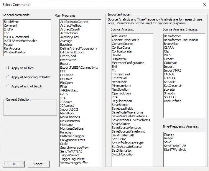
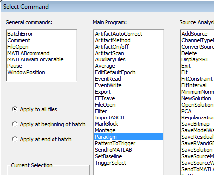
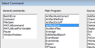
- Press Add Command to add a new command to the batch. The following dialog is opened, showing the available commands:
- Select the desired command and press OK or double-click on the command. A dialog box is opened, allowing to specify individual command parameters.
- If you click on "Apply at beginning of batch" or "Apply at end of batch", the command will only be run at the beginning or the end of a batch. You can use this, for example, at the end of a batch to start a MATLAB script to perform statistics on the results of the batch.
Load and Save Batch
- Press Load Batch to load a previously defined batch or Save Batch to save the current batch to a file (*.bbat).
Load Previous
- Press Load Previous to load the most recently used batch file. Whenever a batch is run, the current set of commands is written to the file Previous.bbat in the Scripts/Batch subdirectory. This file is loaded when you press Load Previous.
Clear All
- Clears all commands from the window.
View Log File
- Each time a batch is run, BESA Research adds information about the batch to a log file, with headings showing the date and time the batch was started. The file is opened automatically in Internet Explorer if errors occurred during processing. Otherwise you may open the file by pressing the View Log File button here or in the dialog that is displayed at the end of batch processing.
- The log file is saved in xml format, and a JavaScript is used to format the display in web browsers. JavaScript should be enabled in the browser to obtain an optimal display of the results. If JavaScript is enabled, the log file is displayed as a list of headings for each batch. Click on a heading to display the results of the corresponding batch.
- To open the log file in the Notepad, hold the Shift key down when pressing the View Log File button.
Batch Command List
- Double-click on a command to edit it. See Batch Commands for descriptions of the dialogs that are opened to edit each command.
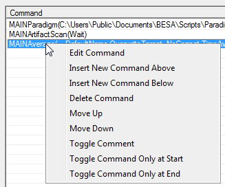
- Right click on a command to open a context menu allowing more options.
- Delete, Move Up, and Move Down can also be applied to multiple selections.
- If you have made a multiple selection, the Del button will delete all the marked commands. Ctrl plus Up or Down cursor keys will move the marked commands up or down.
- Toggle Comment will add or remove a semicolon (;) in front of the command, to deactivate or reactivate the command.
- Toggle Command Only at Start/End will add or remove the text "Start_" or "End_" in front of the command. With these prefixes, the command will only be performed when the first file ("Start_") or the last file ("End_") in the file list is being processed.
Single Step Mode
- Check this item to step through the batch, one command at a time. A dialog is opened after each command, allowing to run the next command, continue the batch without single steps, or stop running the batch. See the “Pause” command for further details.
- During a batch, press and hold down the Pause or Delete key to interrupt the batch and enter Single Step Mode. Press and hold down the Esc key to cancel the batch.
Changes in batch written to database
- Checked by default. If this item is unchecked, file display settings, such as Montage setting and Artifact correction display, are not written to the database. When the file is next opened in BESA Research, the settings made in the batch are not retained.
Leave files in the file list open after running the batch
- If this item is checked, files in the file list will remain open after the batch. This is useful, for instance, if you want to open a set of files, specifying the same montage and/or filter settings for each file.
Press OK to start running the batch. Each command is then applied in succession to each file in the File List.
Note that, while a batch is running press and hold down the Pause or Delete key to interrupt the batch and enter Single Step Mode. Press and hold down the Esc key to cancel the batch.
The log file
A protocol of each batch is written to the log file Scripts/Log/Batch.xml.
When you press the View Log File button, the file is opened in your default browser for xml files. The file will be opened automatically if there was an error during batch processing, unless you have used the BatchError batch command to suppress this behavior.
DHTML formatting of the log file
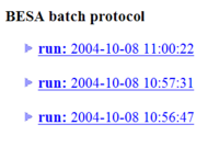
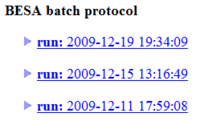
The xml file is formatted using JavaScript (Dynamic HTML). If JavaScript is enabled in your browser, you will first see a list of batch protocol titles, labeled by the date and time at which the batch was started. The most recent batch is at the top of the list.:
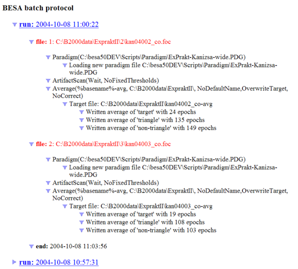
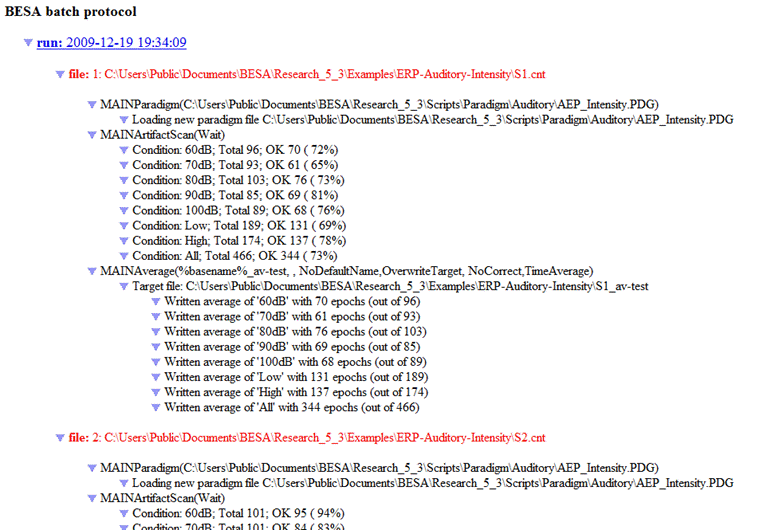
Click on the title to view the protocol for the corresponding batch:
JavaScript and XP Service Pack 2
By default, if the log file is opened in Internet Explorer after XP Service Pack 2 has been installed, IE will warn you with the message: "To help protect your security, Internet Explorer has restricted this file from showing active content that could access your computer". All the protocols in the log file are displayed. You may safely click on the options to allow active content in the log file, if you want to display the file as described above.
Backup of the log file
When the log file is written, a backup of the previous version is written to batch.xml.bak.
If the size of the log file exceeds 200 KB, it is renamed to batch.xml_date_time (e.g. Batch.xml_2004-10-08_10-53-32), and a new version of batch.xml is created.
Placeholders
A powerful feature of the batch commands is the ability to define file names and specify standard paths using placeholders. These are text strings enclosed by percentage (%) signs. They can be used in all batch commands where file names are specified.
Basename
| Placeholder | Description | Example |
|---|---|---|
| %basename% | replaced by the basename of the currently opened file. | If the data file is named "f-spike.fsg", "%basename%-export.fsg" will be interpreted as "f-spike-export.fsg". |
| %basename-n% | replaced by the basename of the currently opened file, but removing the last "n" characters from the name. | If the data file is named "dongle-BB.fsg", "%basename-3%" will be replaced by "dongle", because the last 3 characters of the basename have been removed. |
| %-nbasename% | replaced by the basename of the currently opened file, but removing the first "n" characters from the name. | If the data file is named "BB-dongle.fsg", "%-3basename%" will be replaced by "dongle", because the first 3 characters of the basename have been removed. |
| %orgbasename% | replace by basename of the current file in the file list (it has the same meaning as %basename% if no MAINFileOpen batch command was used in command list) | |
| %base% | replace by basename of the current file without the path | |
| %orgbase% | replace by basename of the current file in the file list without the path | |
| %ext% | replace by extension of the current file | |
| %orgext% | replace by extension of the current file in the file list | |
| %basefolder% | replace by folder of the current file | |
| %orgbasefolder% | replace by folder of the current file in the file list | |
| %t% | Log batch command only: time since start of batch on current file | |
| %T% | Log batch command only: current date and time | |
| %label% | Replace label of the most recent marked block by the block label, not including no. of averages | |
| %LABEL% | Replace label of the most recent marked block by the block label, including no. of averages | |
| %scripts% | replaced by the path to the Scripts folder. | "%scripts%Batch" is where batches are saved by default; "%scripts%MATLAB" is the location of the standard MATLAB scripts used by BESA Research. |
| %montages% | replaced by the path to the Montages folder. | |
| %examples% | replaced by the path to the Examples folder. |
Placeholders for folders
The following placeholders are the same as those used in the [Folders] section of Besa.ini:
The strings enclosed by percent signs (%) are placeholders for the following folders in English-language versions of Windows. Folder names are different for the system and for other language settings. BESA Research will substitute the placeholders by the appropriate folder name for the Windows system and the system language:
- Windows 10 (English)
- Windows 7 (English):
Batch Commands
Batch commands are selected when the "Add Command" button is pressed in the "Batch" Tab. The commands are subdivided into five categories: General commands, commands for the Main module, for the Source Analysis module, imaging commands in the Source Analysis module, and commands for Time-Frequency Analysis. The commands have prefixes, GEN, MAIN, SA, SAIMAGE, and TFC), which identify the category. For compatibility with older program versions, old batches without the prefixes are accepted.
Detailed descriptions of each batch command are available in the electronic help chapter “Batch Processing and Combining Conditions / Batch Processing / Batch Commands”.
General commands - prefixed with "GEN" (can be used anywhere):
| GENBatchError | used to change program behavior when errors occur |
| GENBatchWindowPosition | set the position of the batch window relative to the main window |
| GENComment | comment in the batch script: no batch functionality |
| GENMATLABcommand | send a command string to MATLAB |
| GENMATLABwaitForVariable | tells BESA to wait until Matlab has created a variable with the specified name. |
| GENPause | pause batch operations, allowing step-by-step operations |
| GENFor/GENEndFor | a programming language-like FOR loop |
| GENRunProcess | runs a command line process, e.g. an external program to perform part of the data analysis in the batch |
| GENsaveBitmap | save a screenshot of the Source Analysis or the 3D window |
| SetVariable | the value of the variable is inserted into subsequent batch commands where the text contains the name flanked by % signs |
| GENWindowPosition | set window size and positions to a selection of standard settings, e.g. for bitmap export |
Commands for the Main Module - prefixed with "MAIN":
| MAINArtifactCorrect | run automatic artifact correction |
| MAINArtifactMethod | specify the method for artifact correction |
| MAINArtifactOn | turn artifact correction an artifact view on or off |
| MAINArtifact Scan | run an artifact scan as from the Paradigm Dialog |
| MAINAuxiliaryFiles | associate auxiliary files (e.g. *.ela, *.sfp) with the data file |
| MAINAverage | average the data |
| MAINBaseline | specify the parameters for baseline correction |
| MAINDefineArtifactTopography | define an artifact topography |
| MAINEditDefaultEpoch | edit the default block epoch |
| MAINEventRead | read events from an ASCII event file |
| MAINEventWrite | write events to an ASCII event file |
| MAINExport | export or append data in the selected target format |
| MAINExportToBESAConnectivity | export data segments to BESA Connectivity |
| MAINFFT | calculates the FFT spectrum of the marked data interval |
| MAINFFTmean | starts an averaging procedure which calculates the mean spectral properties in pre-defined regions |
| MAINFFTsave | saves FFT data (generated using the FFT Average option in the Average command) to disk (*.fma) |
| MAINFileOpen | close the current file and open a new file to which the remaining batch commands will be applied |
| MAINFileClose | close the currently open file in a batch, provided it is not the current file in the File List |
| MAINFilter | set filters |
| MAINfMRIArtifact | turns on the fMRI artifact removal |
| MAINGoTo | jumps with the cursor to the specified time point |
| MAINICA | starts ICA decomposition of data on the current screen |
| MAINICAsave | saves selected ICA components as topographies in a file |
| MAINICAselect | opens component selection dialog for managing ICA components |
| MAINImportASCII | import an ASCII file into a *.fsg file. |
| MAINMarkBlock | mark a data block (optionally send to Source Analysis) |
| MAINMarkChannels | mark one or more channels, as given by the list |
| MAINMaxInInterval | within the current marked block, search for the largest absolute value on the specified channel |
| MAINMontage | change the montage (used by the Export command when saving to current montage) |
| MAINParadigm | load a paradigm file |
| MAINPatternToTrigger | convert a tag into a trigger |
| MAINPolygraphicFilters | sets filters for polygraphic or added channels |
| MAINScale | set amplitude and time scales |
| MAINSearchAverageView | start search average view |
| MAINSendToMATLAB | send data to MATLAB |
| MAINSplineConstant | set the spline constant used in spherical spline maps and channel interpolation |
| MAINTriggerRecode | the command recodes a specified trigger number to a new number |
| MAINTriggerSelect | edit the trigger list (cf. Edit / Trigger Values...) |
| MAINTriggerTagDelete | delete one or more triggers or tags |
| MAINViewAverageBuffer | turn on the Average Buffer View and place the specified buffer number to the left in the display |
| MAINViewChannelType | select the channel type to display, and select channel types for mapping, export, etc |
| MAINViewSelected | turns selected view on or off |
General commands for Source Analysis - prefixed with "SA" (but see also MarkBlock, which is used to send a block of data to SA and open the SA window):
| SAAddSource | add a dipole or regional source to a model |
| SAChannelTypeForFit | switch between EEG, magnetometers or axial gradiometers, and planar gradiometers |
| SAConvertSource | convert a source from dipole to regional source, or from regional source to dipole |
| SAcorticalClara | run Cortical CLARA |
| SAcorticalLoreta | run Cortical LORETA |
| SADelete | delete current solution or all solutions, or remove current fit interval or cursor |
| SADICS | start DICS computation (if DICS has been precomputed in the time-frequency image command) |
| SADisplayMRI | switch MRI display on/off and select small or large window |
| SAElectrodeConfiguration</></span> | equivalent to pressing the Org or Std button in the Channel box of the Source analysis window |
| SAExit | close Source Module |
| SAFit | start fit |
| SAFitConstraint | set fit constraints, e.g. Residual Variance, Energy, Maximum Distance, Image Weighting, and their weights. |
| SAFitInterval | set fit or baseline interval |
| <u>SAHeadModel</u> | set the head model |
| <u>SALabelSource</u> | set the label of the specified source number |
| SAMinimumNorm | run a minimum norm analysis |
| SANewSolution | open a new solution |
| SAOpenSolution | open a solution from a file |
| SAPCA | toggle PCA display of data or residual, and transfer a selected number of components to the source model |
| SARegularization | set the regularization values both for discrete and distributed source images |
| SASaveBitmap | save a screenshot of the Source Analysis or the 3D window |
| SASaveLeadfields | save the leadfields of the current source model |
| SASaveModelWaveforms | save model waveforms |
| SASaveResidualWaveforms | save residual waveforms |
| SASaveRVandGFPWaveforms | save residual variance and global field power waveforms |
| SASaveSolution | save the current solution |
| SASaveSourceMontage | save a source montage |
| SASaveSourceWaveforms | save source waveforms |
| SASendToMATLAB | send data, model, source waveforms, images, etc. to Matlab |
| SASetCursor | set the cursor |
| SASetDefaultSourceType | set the default source type (dipole or regional source) |
| SASetOrActivateSource | Turn specified source on or off, or enable/disable source for fitting |
| SASetOrientation | set orientation (of regional source) |
| SASwitchCondition | switch to a specified condition |
Commands for Distributed 3D Volume Images
| SAIMAGEBeamformer | switch between Single Source and Bilateral Beamformer image |
| <u>SAIMAGEBeamformerTimeDomain</u> | start beamformer computation in the time domain |
| SAimageBrainAtlas | turns on the Brain Atlas overlay on volumetric image |
| SAIMAGECLARA | generate CLARA image |
| SAIMAGEClip | clip image values under a threshold |
| SAIMAGEExport | save the results of minimum norm or 3D imaging method |
| SAIMAGEGotoMax | set the crosshair cursor at the nth maximum in the image |
| SAIMAGEImport | load a 3D volume image from file |
| SAimageImportFMRI | import fMRI image to Source Analysis Module |
| SAIMAGELAURA | create LAURA image |
| SAIMAGELORETA | create LORETA image |
| SAIMAGESLoreta | create sLORETA image |
| SAimageSESAME | start SESAME computation |
| SAIMAGESSLOFO | create SSLOFO image |
| SAIMAGEUser-Defined | create user-defined image |
| SAIMAGESaveLeadfields | save the leadfields of all the voxel sources in a 3D image |
| SAIMAGEClip | clip current 3D image |
| SAIMAGESmooth | smooth current 3D image |
| SAIMAGESetCrosshair | set the position of the crosshair in the 3D image |
Commands for Time-Frequency Analysis (TFC)
| TFCStartTFAnalysis | (previously TFCgo) start TFC analysis using the current paradigm settings |
| TFCdisplay | change the TFC display (e.g. power/amplitude, coherence) |
| TFCsave | save numerical results to an ASCII file, or save a screenshot of the TFC window |
| TFCimage | start beamformer analysis on a selected time-frequency range |
| TFCSendToMATLAB | send TF results or single-trial data to MATLAB |
How to Average Your Data in a Batch
Using batch processing, several files from an experiment can be averaged at a time.
Here we summarize the steps required:
Before running the batch
- Create the paradigm, and save the paradigm file.
- Open each individual data file to check the data:
- Make sure auxiliary files are defined and loaded properly, and the data are displayed correctly.
- Eyeball the data.
- Define bad (and interpolated) channels.
- Mark artifact time ranges.
- If required, set up artifact correction for the file.
- The data file can be closed again after this step.
Preparing the batch
- Open at least one file and select Process / Batch Scripts.... The file(s) should be displayed in the file list. Alternatively, just select Process / Batch Scripts..., and add the files by
- pressing the Add File button
- dragging the files from Windows Explorer
- Opening a previously saved list with Load File List
- You can delete files from the list (press Del) or edit the file sequence using the right click context menu.
- Select the Batch Tab.
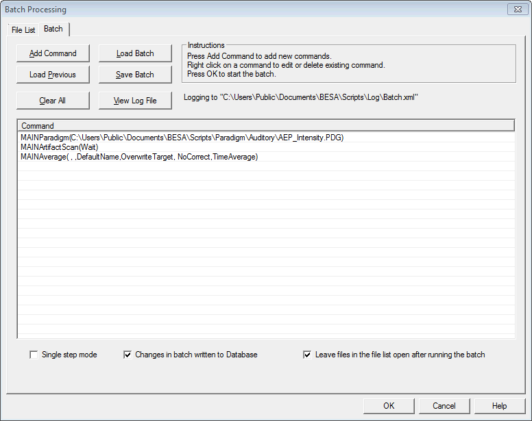
- Add commands to your script. For averaging, these would normally be
- Paradigm -- to load the paradigm file
- Artifact Scan -- to run the artifact scan
- Average -- to perform the average
- Save these commands (press Save Batch).
- Test the commands on the files in the current file list: press OK
- Look at the log file (press View Log File) to check the results of averaging.
- Look at the data averages to make sure they have been done correctly.
- Repeat these steps until averaging is working properly.
Running the batch
- Select Process / Batch Scripts....
- Open the files you want to average in the batch in the file list:
- Any files that were open in BESA are included in the list
- Files can be added using the Add File button
- You may drag one or more files from Windows Explorer to the file list
- Alternatively, load a previously saved file list.
- Edit the file list, e.g. delete unwanted files (use the Del key or the right click context menu), or reorder the files (use Ctrl + cursor keys or context menu).
- Note that the order of files in the list specifies the order in which they will be processed in the batch script. This order will be important if all results are saved to the same target file. Otherwise the file sequence is not important.
- Optionally, save the file list (press Save Batch
- Select the Batch Tab, and load the previously defined batch script with Load Batch.
- Press OK to run the batch.
How to Merge and Compress raw data
Using the Export command in a batch, several data files can be merged into a single data file in BESA's data format (*.foc).
This can be useful if data from one subject have been collected in several data blocks, and you want to analyze all data blocks together.
Optionally, to save space, data can be saved in compressed format.
Files can be merged:
- if they have identical channel configurations, or
- there are at least 16 EEG channels, and the export format is Standard 81 (i.e. EEG channels are interpolated to 81 standard locations).
How to merge files:
- Select Process / Batch Scripts...
- Add all the files that are to be merged to the file list:
- Any files that were open in BESA Research are included in the list
- Files can be added using the Add File button
- You may drag one or more files from Windows Explorer to the file list
- Alternatively, load a previously saved file list (Load File List).
- Rearrange the files in the file list to the sequence in which they should be merged.
- Select the Batch Tab and insert an "Export" command, as described below.
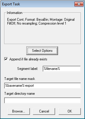
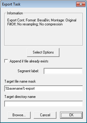
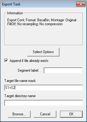
The following dialog shows a possible configuration of the Export command:
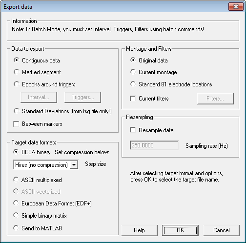
- The parameters shown in the Information box are the settings chosen in the Export Dialog when the Select Options button has been pressed.
- Append if file already exists must be checked in order to merge the files.
- The target file name must be fixed, i.e. don't use the %basename% variable, because that will result in a different target file name for each source file.
- There are two variables that can be used for the segment label:
- %filename% will insert the basename of the source file into the segment label.
- %c% will insert the file number into the segment label. The number gives the position of the file in the file list. For instance, "File %c%" will generate the label "File 2" for the second file in the list.
Example: Data averaging in the auditory intensity experiment
In this example, two raw data files, s1.cnt and s2.cnt, from the auditory intensity experiment will be batch averaged.
Please note that there are further tutorials covering this experiment. The first file is contaminated by many eyeblinks, and more epochs would be averaged if eye correction were used (see Viewlet demonstration on artifact correction on the BESA website). However, in this tutorial we will just use artifact rejection.
A. Various ways of creating a File List
1. Files that were open in BESA Research are automatically added to the File List. Start BESA Research and open the files s1.cnt and s2.cnt in the directory Examples\ERP-Auditory-Intensity.
2. Select Process / Batch Scripts.... You should see the file names in the File List Tab something like this:
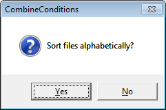
3. You can resort the files in the file list alphabetically by clicking onto the File List column header:
Alternatively, you can mark any file, hold down the Ctrl key and press the Up or Down arrow to move the file name up or down the list. This is the sequence in which files will be processed in the batch.
4. Press Save File List and save the list you have created to ERP-Aud-Ex1.flist.
5. Highlight both names and press the Del button to remove them from the list.
6. Files can be dragged from Windows Explorer. Start Windows Explorer and navigate to the ERP-Auditory-Intensity subdirectory of your BESA Research examples folder (located in the Public Documents folder of your computer). Click on s1.cnt and drag it with the mouse onto the File List Tab. Let go of the mouse. BESA Research opens the file, and displays the name in the File List. Repeat for s2.cnt.
7. Highlight both names and press the Del button to remove them from the list.
8. Files can be added using the Add File button. Press Add File and navigate to the Examples\ERP-Auditory-Intensity subdirectory. Select s1.cnt. Press Ctrl and select s2.cnt. Both names should then be displayed in the File Open dialog. Press OK to add the files to the file list.
9. Highlight both names and press the Del button to remove them from the list.
10. Files can be loaded from a previously saved file list. Press Load File List and select ERP-Aud-Ex1.flist, the list you saved in step 6 above.
B. Setting up the batch
1. We will add three commands, Paradigm, Artifact Scan, and Average, to create a batch that will be applied to the two files in the file list.
2. Click on the Batch Tab.
3. Press the Add Command button to obtain the Select Command window:
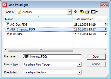
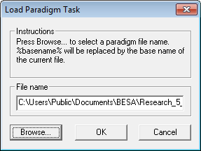
4. Click on Paradigm and then on OK (alternatively, double-click on Paradigm). Hit Browse, navigate to the Auditory folder, and select AEP_Intensity.pdg, the paradigm for the auditory intensity experiment.
5. Press OK to obtain the Load Paradigm Task window.
6. Press OK, and the first task in the batch is ready, and listed in the Batch Command window. If you want to modify the command, double-click on it to open the above window, that allows to browse for a different paradigm file.
7. Next, we add the Artifact Scan command. Click on the Add Command button, and select Artifact Scan.
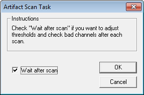
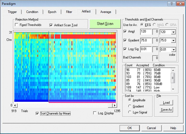
8. Press OK to open the Artifact Scan Task window. We want to be able to view the results of the scan, and adjust thresholds and bad channels if necessary. Therefore, check the Wait after scan checkbox.
9. Press OK to close the Artifact Scan Task window. Our batch now contains two commands.
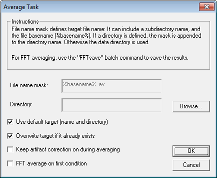
10. Finally, we will add an Average command. Press the Add Command button and select Average. Press OK to open the Average Task window.
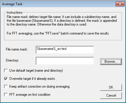
11. With the default settings, the average would be saved to the same directory as the data. The file name mask is set by default so that in this example the two averages would be saved to s1-av.fsg and s2-av.fsg. We will save the averaged files to subdirectory "Averages" of the data directory. Uncheck the Use default target check box, change the File name mask to %basename%_av-test in order not to overwrite the predefined files.
12. Press OK to close the Average Task window. Our batch is now complete.
13. We will now save the batch so that it can be used again. Press the Save Batch button, and save to the file ERP-Aud-ex1.bbat. Note that an easy way to generate new averaging batches is to load a previously save batch and edit the commands -- it may only be necessary to edit the Paradigm command to select the relevant paradigm file, and maybe to adjust the target directory in the Average command.
14. Press OK in the Batch Window to start the batch running. As requested, the batch pauses after the artifact scan:.
You may now adjust the number of rejected trials, e.g. by moving the vertical red bar to the left, or exclude bad channels.
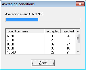
15. Press OK to continue with averaging.
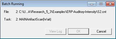
16. Note that, in the background, the Batch Running window is providing feedback about the current file and current task.
17. The batch will stop again after the next artifact scan. Press OK to allow the batch to run to the end.
18. Press View Log to view the batch protocol. If you are using Internet Explorer or Netscape family (Mozilla, Firefox) browsers, and JavaScript is enabled, you will first see just batch titles defined by the date and time the batch was started. The most recent title is at the top of the list. For other browsers, or if JavaScript was not enabled, all protocol texts are expanded as in 19 (below).
19. Click on the first title to expand its protocol. Here, for example, the protocol gives feedback about the number of epochs that were averaged for each file.
20. Finally, press OK to return to the main BESA Research display. Open the averages in the Averages subdirectory to confirm that they were generated properly.
Example: Merging files using the Export Command
Here we will demonstrate the use of the Export command to merge two files. We will combine the two averages from the previous example (Data averaging in the auditory intensity experiment) into one target file.
A. Generate the file list
- Start BESA Research and load the two data files S1_av-test.fsg and S2_av-test.fsg that were saved in the previous example.
- Select Process / Batch Scripts....The two file names should be displayed in the file list.
- In the file list, make sure that s1_av-test.fsg is the first file in the list. If it is not, highlight the file, and move it up using Ctrl+up, or right click and select Move Up in the context menu.
B. Generate the batch
1. Press the Add Command button, and select the Export command.
2. Press OK to open the Export Task window.
3. Press the Select Options... button to open the Export Dialog.
4. Since we are combining averages, select Hires (no compression) in the Target data format drop-down list (If we were merging raw data files, it is better to select compression. Press OK to close the dialog. Check Append if file already exists, so that the files will be merged. Enter s1+s2 in the target file name mask edit box. This ensures that both files will be saved to the same target: S1+S2.fsg.
5. Press OK to close the Export Task window. The Export command is displayed.
6. Optionally, you may save the batch file by pressing Save Batch.
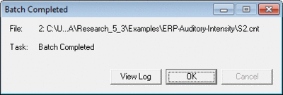
7. Press OK to run the batch, and OK in the Batch Completed window to return to the BESA main window.
8. Finally, open the file S1+S2.fsg to confirm that it contains the two merged files.
C. Merge raw data
- Repeat the above task to merge the two raw data files S1.cnt and S2.cnt into a single target file S1+S2.foc. In this case, select one of the compression options as the target data format. Note that you would not normally want to merge two files from different subjects. However, several data blocks from the same subject can conveniently be merged using this method.
Note that *.fsg files can also be merged using the Combine Conditions dialog.
Combine Conditions, Channels
Combine Condition Scripts
With the Combine-Conditions module you can do a variety of operations on BESA averages (files with the extension *.fsg, and other segment files, such as *.mul, *.avr, *.swf):
- Create grand averages
- Combine averages (add, subtract, weighted/unweighted)
- Merge files
- Exclude unwanted averages
- Rename conditions
- Rename or resort channels
- Generate averages or differences over selected channels
- Transform the data: standard interpolated 81 electrodes, change sampling rate, change interval
- Determine peaks, mean amplitudes, or integrals on data averages
- These operations can be performed on one or more files simultaneously. Results of an operation are stored in a single target file.
The module includes four tabbed windows:
- File List: Define a list of files on which the operations will be performed.
- Condition List: List the condition names, define target condition names, and how input conditions are combined into target conditions.
- Channel List: List the channel names, define target channel names, and how input channels are combined into target channels.
- Run Scripts: Define global options for the output (e.g. spatial interpolation, resampling, copy/merge or average, peak analysis). Start the operation.
- Note that in all four tabs, configurations can be saved for future use, and the Load Previous button restores the most recently used configuration.
Condition List Tab
List the condition names, define target condition names, and how input conditions are combined into target conditions.
The first column of the list box shows a list of all the condition names found in the source files.
Rows of the list box define the source conditions. Columns define the target conditions.
Initial setting
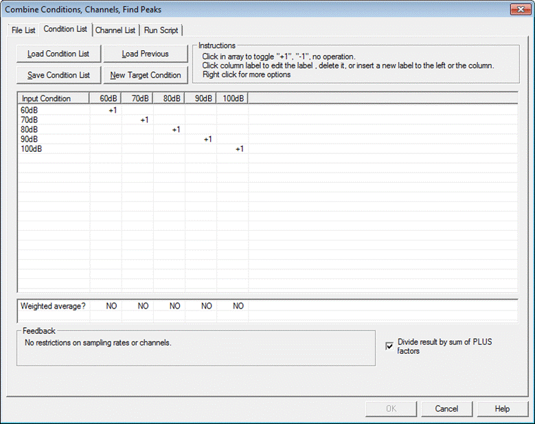
When first selecting the tab, each column shows each condition name found in the source files (as in the example below). In the list box, there is a "+1" along the diagonal. The result of this selection is that target conditions will have the same name as source conditions. Right click on source condition labels to view properties (e.g. no. of samples, time range, sampling rate).
Editing the condition list
- Target condition names can be edited, inserted or deleted by clicking on the label at the top of each column.
- Click on a box within the list to toggle between "+1", "-1" and blank. These correspond to the operations:
- "+1" = add
- "-1" = subtract
- blank = do nothing
- Right click on a box for further operations: conditions can be weighted by a given factor other than 1.
Divide result by sum of PLUS factors
- Normally, when creating an average over conditions, the sum is divided by the number of conditions, or a weighted average is generated (see below). If "Divide result by sum of PLUS factors" is unchecked, the conditions will be summed rather than averaged.
- Note that, when making differences between conditions, no such division is required. BESA Research will uncheck the checkbox automatically if subtraction ("-1") is specified somewhere in the condition list.
Weighting of averages
- Below the list, click on the Weighted Average row to toggle "YES" and "NO". "YES" means that averages will be weighted by the number of epochs contributing to the average. For instance, if average A contained 100 epochs and average B contained 200 epochs, the weighted average will be computed as
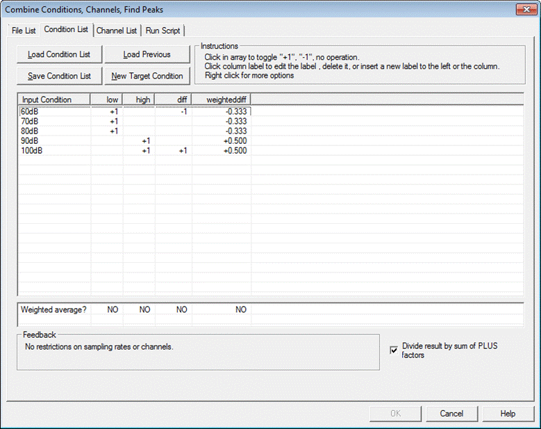
- Values other than +1 or -1 in the boxes apply a different kind of weighting. For instance, we want to compute the difference between the means of conditions A, B, C and D, E. Use a right click to specify the fraction 1/3 for each of A, B, and C, and -1/2 for each of D and E (see example below).
Save the current condition list
- Press the Save Condition List button.
Load a condition list
- Press the Load Condition List button.
Load previous settings
- Press the Load Previous button
Feedback
- Conditions that have different numbers of electrodes (averaging across different files) can only be combined if channels are interpolated to a standard set of electrodes.
- Conditions that have different durations or sampling rates can only be combined if the sampling rate and durations are made the same.
- Feedback about the above situations is displayed by the presence of tick marks above the list box.
Channel List Tab
List the channel names, define target channel names, and how input channels are combined into target channels.
Note that this tab is very similar in usage to the Condition List Tab. Note also that some of the functions performed in this tab could also be done in the Montage Editor. It may be a matter of convenience whether you choose to perform these operations here or in the Montage Editor.
The first column of the list box shows a list of all the channel names found in the source files.
Rows of the list box define the source channel. Columns define the target channel.
Initial setting
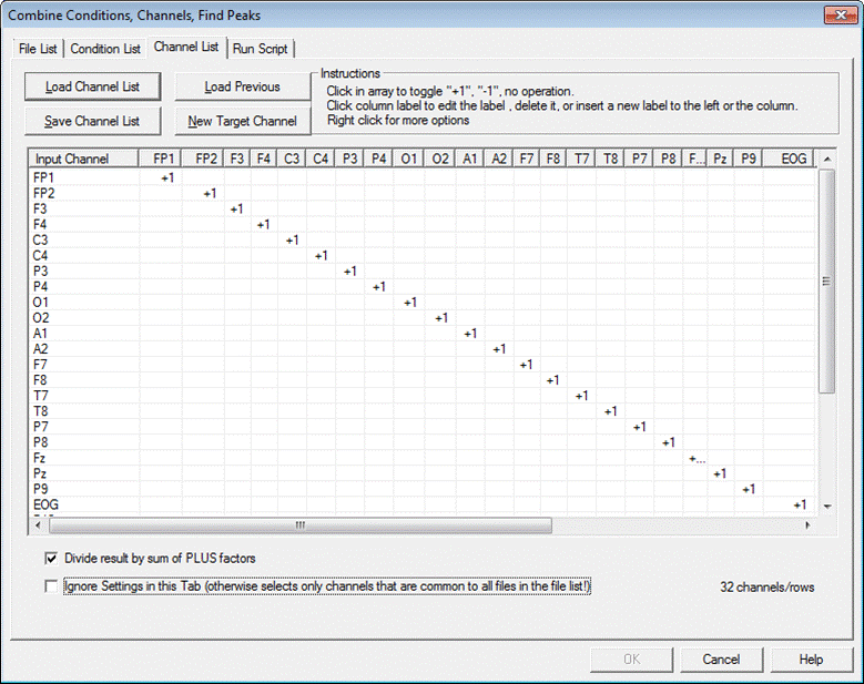
When first selecting the tab, each column shows each channel name found in the source files (as in the example below). In the list box, there is a "+1" along the diagonal. The result of this selection is that target channel will have the same name as source channel.
Combining files
If files with different channel configurations are included in the File List, the rows and columns of the Channel List Tab will only contain the labels for the channels that are in common among the files.
If the files in the File List have a different sequence of channels, the sequence of the first file in the list will be adopted in the Channel List.
Thus, for the initial setting, unless the "Ignore Settings in this Tab" checkbox is checked, the target grand average or peak/amplitude analysis, etc. will be applied using only channels that are in common among the input files, and using the channel sequence of the first file in the File List. By changing the target channels or by changing the entries in the Channel List, new channels consisting of averages or differences can be generated.
What can the Channel List be used for?
Some examples:
- Reorder or relabel channels
- Create channel differences
- Create averages over channel groups, e.g. for peak analysis
- Extract a selection of channels for peak analysis or mean amplitudes
- Create grand averages across files with different channel configurations, just using channels in common among the files
Editing the channel list
- Target channel names can be edited, inserted or deleted by clicking on the label at the top of each column.
- Click on a box within the list to toggle between "+1", "-1" and blank. These correspond to the operations:
- "+1" = add
- "-1" = subtract
- blank = do nothing
- Right click on a box for further operations: channels can be weighted by a given factor other than 1.
Divide result by sum of PLUS factors
- Normally, when creating an average over channels, the sum is divided by the number of channels, or a weighted average is generated (see below). If "Divide result by sum of PLUS factors" is unchecked, the channels will be summed rather than averaged.
- Note that, when making differences between channels, no such division is required. BESA Research will uncheck the checkbox automatically if subtraction ("-1") is specified somewhere in the channel list.
Save the current channel list
- Press the Save Channel List button.
Load a channel list
- Press the Load Channel List button.
Load previous settings
- Press the Load Previous button
Run Scripts Tab
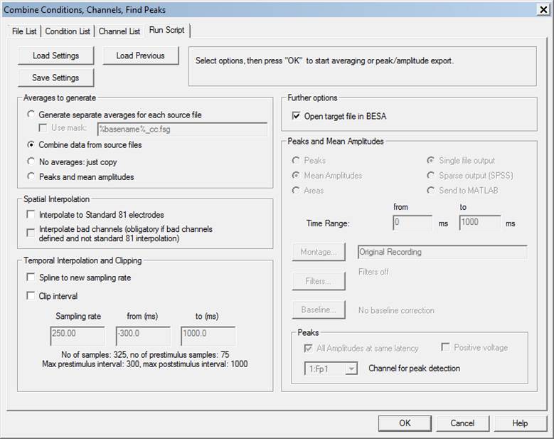
Define global options for the output (e.g. spatial interpolation, resampling, copy/merge or average, peak detection. Start the operation.
Load or Save Settings
- You can save the current settings of this tab to a file (*.run) which can be loaded later.
- When you run the script, the current settings are saved automatically to a file "PreviousSettings.run".
Load Previous
- Press this button to load the previous settings (from "PreviousSettings.run").
Averages to Generate
- Generate separate averages for each source file. Averages are performed over conditions within the source file, and are then appended to the target file.
- Combine data from source files. Conditions are combined over all source files into a single target average.
- No averages, just copy. Files are copied and merged to the target file. Use this option for renaming conditions, merging files, removing unwanted averages (see below), changing the sampling rate and interval.
- Peaks and mean amplitudes. Specify time ranges for peaks, mean amplitudes, or integrals (areas).
- Note: When generating or copying averages (first three options), filters and baseline settings are turned off. For Peaks and mean amplitudes, filters and baseline settings are specified in the dialog.
Spatial Interpolation
- Interpolate to Standard 81 electrodes. The target file will contain only electrodes (other channels are omitted), using the Standard 81 configuration (as in other export functions within BESA Research). This cannot be selected if the source data contain less than 16 EEG channels.
- Interpolate Bad Channels. Bad electrode channels in the source file will be interpolated. If the above option is deselected and bad channels exist in one or more of the source files, this option is always on.
BESA Research can interpolate EEG, and MEG if the sensors are axial gradiometers or magnetometers. If other channels are marked as bad in one or more of the source files, these will be defined as bad in the target file. This applies to MEG planar gradiometers, to polygraphic data, and to ICR channels.
Temporal Interpolation
- Spline to New Sampling Rate and Interval. Data can be converted to a new sampling rate, and the interval can be changed.
- If the sampling rate is reduced, the data will be low-pass filtered at 1/3 sampling frequency before reduction.
- If the sampling interval is changed, the prestimulus and poststimulus intervals are limited by the smallest intervals in the conditions contributing to the averages. These limits are shown below the edit boxes.
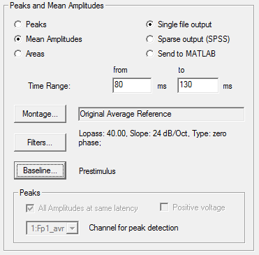
Peaks and Mean Amplitudes
Peaks:
- Select the time range between which peaks are to be determined.
- Select the montage on which the peaks are to be determined.
- Define the filter settings.
- Define the baseline settings.
- Specify whether peaks are to be defined at one latency: if so, select the channel on which peaks are to be detected.
- Specify whether you want to find positive or negative peaks.
Mean amplitudes and areas:
- Select the time range over which the mean amplitudes or areas are to be determined.
- Select the montage on which the mean amplitudes or areas are to be determined.
- Define the filter settings.
- Note that when computing areas, data are first rectified (made positive) and then summed over the time range.
Output options of the analysis:
- A single ASCII file that contains the result of the analysis for all data sets, conditions, and channels including header and information lines.
- A sparse output suitable for import in SPSS. Each variable (e.g. a latency, a channel amplitude) constitutes one column of the output file.
- Direct transfer to MATLAB into a struct besa_peak. For more information on the data transfer from BESA Research to MATLAB, please refer to help chapter “The MATLAB interface”.
Starting the Operation
- Press OK to start the operation. After the operation is completed, and the "Open target file in BESA" box is checked, BESA Research will open the target file. "Open target file in BESA" cannot be checked if "Peaks and mean amplitudes" was selected - then the result of the operation will be an ASCII file or a MATLAB transfer.
- You will be asked for the name of the target file (unless a MATLAB transfer of peak data has been performed).
Restrictions
- Depending on source file configurations, not all options above are selectable. For instance, if two files contain different numbers of electrodes, and the "Ignore Settings in this Tab" checkbox is checked in the Channel List Tab, spatial interpolation to Standard 81 is enforced in the target. Similarly, if different sampling rates are used in different files, temporal interpolation is enforced.
- You are not allowed to add files to the file list if the channel configuration is different, and the data cannot be combined with Standard 81 interpolation. Since Standard 81 interpolation is only possible for EEG, multiple files without EEG can only be loaded if they have the same number of channels.
How to Create Grand Averages
- Open the files you want to average in BESA Research.
- Start the Combine Conditions Module (ERP / Combine Conditions...).
- Click on the Condition List Tab. By default, the target conditions receive the same name as the source conditions. To average across different conditions, click in the list boxes to obtain "+1" for each source condition to combine, and rename the target condition to define a meaningful name for the average.
- Click on the Run Scripts Tab.
- If you have more than one file, specify whether averages should be generated across files (Combine data from source files) or within files (Generate separate averages for each source file).
- Select other options if required (spatial or temporal resampling).
- Press OK.
How to Generate Differences Between Conditions
- Open the files you want to operate on in BESA Research.
- Start the Combine Conditions Module (ERP / Combine Conditions...).
- Click on the Condition List Tab. By default, the target conditions receive the same name as the source conditions. To create differences, click in the list boxes to obtain "+1" for one of the source conditions, and "-1" for the source condition to subtract, and rename the target condition to define a meaningful name for the difference.
- Click on the Run Scripts Tab.
- If you have more than one file, specify whether averages should be generated across files (Combine data from source files) or within files (Generate separate averages for each source file).
- Select other options if required (spatial or temporal resampling).
- Press OK. An average of the differences is generated. If only one example of each condition exists, e.g. in a grand average file, the result is the difference between conditions.
How to Merge Files
- Open the files you want to merge in BESA Research.
- Start the Combine Conditions Module (ERP / Combine Conditions...).
- Click on the Condition List Tab. By default, the target conditions receive the same name as the source conditions.
- Click on the Run Scripts Tab. Select "No averages, just copy".
- Press OK.
Notes
- If the source files have different electrode configurations, use the Standard 81 configuration for the target.
- If the source files have different sampling rates or intervals, use Temporal Interpolation.
How to Remove Unwanted Averages
Removing one or more unwanted segments
- Normally, all conditions are read from a source file. To exclude one or more segments from operations in the Combine Conditions module, mark the segments as artifacts in the main program display. It is sufficient for the beginning or the end of an artifact interval to be within the segment for the segment to be excluded.
- Open the file you want to operate on in BESA Research.
- Start the Combine Conditions Module (ERP / Combine Conditions...).
- Click on the Condition List Tab. By default, the target conditions receive the same name as the source conditions.
- Click on the Run Scripts Tab. Select "No averages, just copy".
- Press OK.
- The target file contains the copied data without the conditions that were marked as averages.
Removing one or more unwanted conditions (by label)
- Open the file you want to operate on in BESA Research.
- Start the Combine Conditions Module (ERP / Combine Conditions...).
- Click on the Condition List Tab. By default, the target conditions receive the same name as the source conditions.
- Deselect the target conditions you want to omit (replace the "+1" by a blank).
- Click on the Run Scripts Tab. Select "No averages, just copy".
- Press OK.
- The target file contains the copied data without the conditions that were marked as artifacts.
How to Rename Conditions
- Open the file you want to operate on in BESA Research.
- Start the Combine Conditions Module (ERP / Combine Conditions...).
- Click on the Condition List Tab. By default, the target conditions receive the same name as the source conditions. Click on column headings to rename the target conditions.
- Click on the Run Scripts Tab. Select "No averages, just copy".
- Press OK.
- The target file contains the copied data with the renamed conditions.
How to Change the Sampling Rate
- Open the file(s) you want to change in BESA Research.
- Start the Combine Conditions Module (ERP / Combine Conditions...).
- Click on the Condition List Tab. By default, the target conditions receive the same name as the source conditions.
- Click on the Run Scripts Tab. Select "No averages, just copy".
- Select "Spline to New Sampling Rate and Interval" and type the new sampling rate into the edit box.
- Press OK.
Example: Create grand average and combinations of conditions
In this example, we will generate a grand average of the results of the Auditory Intensity Experiment. The experiment includes averages from five different stimulus intensities. We will create a grand average over each intensity, but also include means over the two lowest and the two highest intensities, and the difference between these two combinations.
A. File selection
- Start BESA Research and open files S1_av.fsg - S10_av.fsg in the Examples\ERP-Auditory-Intensity folder. The files contain the individual averaged data of the 10 subjects who participated in this study.
- Select ERP / Combine Conditions... The file list should display the two files, with feedback about the number of averages and conditions. 8 epochs are found. See the “Data averaging in the auditory intensity experiment” example for examples how to manipulate the file list.
B. Define conditions
1. Click on the Condition List Tab. The initial window defines target conditions with the same name as the source conditions. To generate the grand average over these conditions we could proceed without further changes to the Run Scripts Tab. However, we want to modify the condition list and create a condition that contains the grand averaged difference between the High and Low conditions.
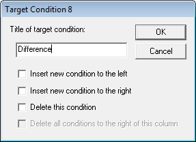
2. Click on the All column label. In the resulting window, rename condition All to Difference. Then press OK.
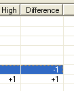
3. The last column is now labeled Difference. Left-click twice onto the ‘+1’ entry that links this condition to the All input condition. This will remove the link and leave the field blank. To define the ‘Difference’ condition as the average of ‘High’ minus ‘Low’ over subjects, left-click once into the field linking input High with target Difference to generate an entry ‘+1’ in this field. Left-click twice into the field linking input Low with target Difference to generate an entry '-1’.
4. Press Save Condition List and save the list to ERP-aud-ex1.clist. This condition combination can thus be loaded later using the Load Condition List button.
C. Run the script
- Click on the Run Script Tab.
- The default tab settings are ready for generating the grand average (Combine data from source file and Open target file in BESA should be checked). Just press OK. Enter All_Subjects_cc-test.fsg as file name and press Save.
The resulting file contains the 8 target conditions, 60db, 70dB, 80dB, 90dB, 100dB, Low, High, and Difference.
Example: Average files from different experiments
This example is intended to illustrate several features of the Combine Conditions Dialog, such as electrode interpolation and resampling. We will combine an average from the Auditory Intensity experiment with one from the P300 auditory experiment. In this particular case, it is not a very meaningful thing to do, but it shows what is possible. For instance, the same experiment may have been performed using different sampling rates or electrode combinations. This example shows how such data may be combined.
A. File selection
- Start BESA Research and open the file All_Subjects_GA.fsg in the Examples\ERP-Auditory-Intensity folder. The file contains the grand average data from the auditory intensity experiment.
- Open the file RareFrequentResponseLeft.fsg in the Examples\ERP-P300-Auditory folder. This file contains averages from the P300 auditory experiment.
- Select ERP / Combine Conditions... Note that the files have different sampling rates and different numbers of electrodes.
B. Define conditions
1. Click on the Condition List Tab. Note that the feedback text at the bottom of the window displays the text "Standard 81 interpolation required to generate average; Across files: resampling or change in time range required to generate average". The condition labels show all the names from both files.
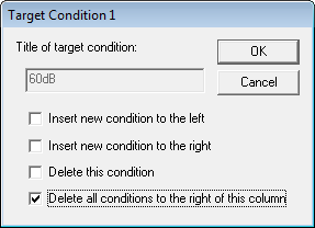
2. We will exclude most conditions, and just combine the most similar conditions from the two experiments: the "Standard" and the "80dB" conditions. Click on the title of the first column, Blink. Select “Delete all conditions to the right of this column”, and press OK.
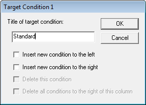
3. Click on the title again, and rename the target condition to "Standard".
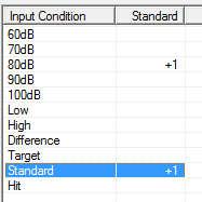
4. Click twice in the first line to remove the "+1" entry there. Click once in the third row ("Frequent"), and in the 7th row ("80dB"), to display "+1" at each entry. Thus, just two of the conditions will be combined into one target condition.
C. Run the script
1. Click on the Run Script Tab.
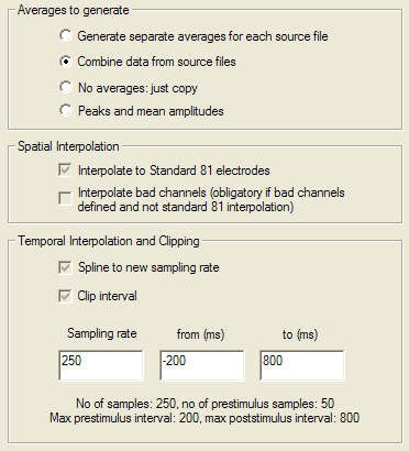
2. Note that Interpolate to Standard 81 electrodes is checked and grayed: since two different electrode sets are to be combined, we can only do this by interpolating electrodes. Also, both Spline to new sampling rate and Clip interval are checked and grayed. Again, these settings are required in order to be able to average the two data files together. The sampling rate is set to the higher of the two selections. The time range is set to the largest possible range that can be clipped from the two data sets. For now, leave these settings as they are, and press OK. Save the target to TestCombineExpts_CC-std81.fsg.
| Review | |
|---|---|
| Source Analysis | |
| Integration with MRI and fMRI | |
| Source Coherence | |
| Export | |
| MATLAB Interface | |
| Special Topics | |
