Source Coherence How to...
Contents
Source Coherence: How to...
How to Start the Beamformer from the Time-Frequency Window
This chapter shows how to start the BESA Multiple Source Beamformer from the time-frequency window. The displayed screenshots are taken using the file BESA5/Examples/Learn-by-Simulations/AC-Coherence/AC-Osc20.foc (see BESA Tutorial 6: "Tutorial on source coherence" on our website http://www.besa.de).
The time-frequency beamformer is especially useful to image induced oscillatory activity in- or decrease. Induced activity cannot be observed in the averaged data, but shows up as enhanced averaged power in the TSE (Temporal-Spectral Evolution) plot.
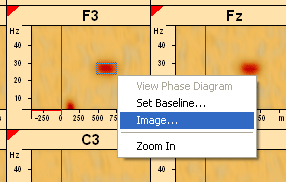
In the time-frequency diagram of any channel, left-drag to mark a time-frequency region of interest, e.g. a region of power increase. When the left mouse button is released, select 'Image' from the popup menu.
Note: The current montage and the type of time-frequency plot currently displayed (TSE, amplitude/power, Coherence) does not affect the output of the beamformer image, because the image is always based on the complex single-trial spectral density of the original recording montage. The status of the 'subtract average signal' button is considered, however. This allows to image either evoked and induced activity or induced activity only.
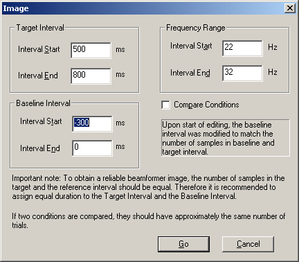
The 'Image' edit window is displayed. It allows for adjusting the time-frequency range of the target interval and for a re-definition of the baseline interval. If a control condition has been specified, you can choose to reference the power in the target time-frequency interval to the corresponding interval in the control condition instead of the baseline interval by checking 'Compare Conditions'.
Note: The text within the window emphasizes that it is recommended to use the same duration for the Baseline Interval and the Target Interval to obtain a reliable beamformer image. The reason is the dependence on the noise estimate on the number of trials that enter the covariance matrix computation. The same recommendation holds if two conditions are compared: It is recommended to define conditions such that they contain approximately the same number of trials. If the baseline interval defined in the Time-Frequency window (the red bar on the x-axis) is larger than the target time interval specified by the dragged rectangle, the baseline interval in the 'Image' dialog window is automatically shortened to match the duration of the Target Interval. If for some reason these requirements cannot be met, it is recommended to compute a beamformer image with regularization. This is achieved by adjusting the SVD cutoff in the Source Analysis window using the menu entry 'Image/Settings'.
Press the 'Go' button to start the beamformer computation.
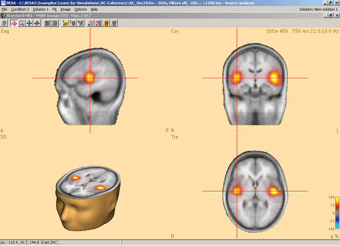
BESA Research now computes mean time-frequency covariance matrices for the target and the reference interval. The source analysis window opens with an enlarged 3D imaging display that compares the power in the target and the reference interval as computed with a bilateral beamformer. The result is superimposed onto the individual or standard MRI.
For more information on the multiple-source beamformer (MSBF), please refer to chapter "Source Analysis".
How to Start DICS computation from the Time-Frequency Window
How to create DICS images you will find in the chapter “Source Analysis / 3D Imaging / Dynamic Imaging of Coherent Sources (DICS)”.
How to Compute Time Lags between oscillations using Phase Diagrams
The phase diagram option is used to analyze phase differences between coherent channels. This can give an insight into a possible coupling of brain regions which may be necessary e.g. to integrate input from various specialized neurons to a common perception. However, the measured coupling is also influenced by volume conduction effects (scalp coherence) or the modeling parameters (source coherence).
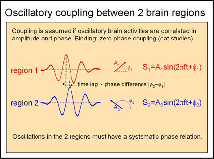
If brain regions show oscillatory coupling in the same frequency range, the phase relationship should be constant over some time:
Since we cannot obtain an ideal frequency resolution using a time-frequency transform, any oscillation frequency is smeared out over several sampling frequencies in the transformed signal. If the delay between the two oscillations is constant, the phase shift between the signals rises linearly with the frequency. We can get a precise estimate of the delay if we use several neighboring frequencies for the calculation. Practically, you can achieve this by the following steps:
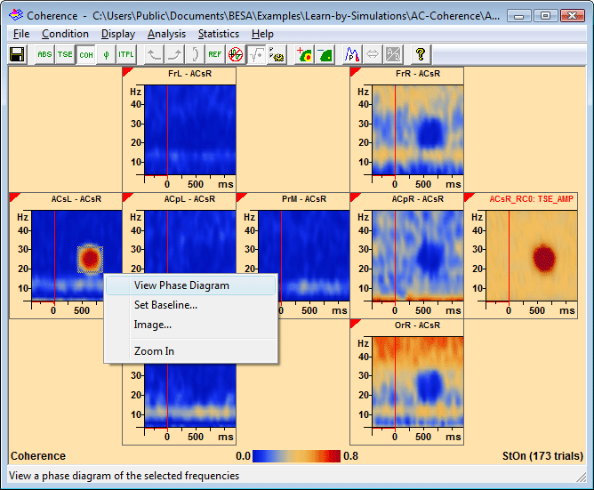
1. Enter coherence mode, either by double-clicking on the channel of interest, or by right-clicking on it and selecting coherence from the popup menu.
2. In a coherence plot, drag over an area of interest which comprises the time interval where the oscillation occurs and the relevant frequency range. The left-mouse popup menu appears (see the leftmost channel termed ACsL in the example below):
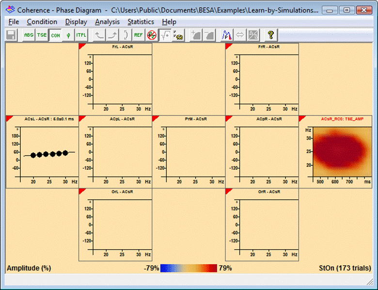
3. Select the menu entry 'View Phase Diagram'. In all channels where coherence was shown previously, the plot changes to display the phase diagram. Inside the marked time-frequency region, the mean phase difference ϕi within the time window is calculated for each frequency νi, and the values are plotted. The phase is calculated from the cross-spectral matrices of the single trials. The error bars shown in the display are the standard deviations of the phase over the time.
The time lag is calculated from a regression fit to the values. The fitting procedure takes phase shifts of π into account, which can occur due to volume currents, or due to dipole orientations. First, a straight line is fitted to the data. Then, one of two different approaches are used to compute the time lag, depending on the characteristics of the values.
- If extrapolation of the line to ν= 0 Hz yields a phase difference of approximately 0 or approximately π, or if a zero crossing at the origin is within the error margins of the fit, the delay can be calculated directly from the data values. For each data value, the relationship ∆ti = ϕi/ (2π νi) holds. The time lag is calculated as the weighted mean, where the weights are given by the individual errors of fi (the errors are given by the standard deviation over the time samples).
- If the regression line does not cross the origin, the gradient of the fit is used to calculate the time lag as ∆t=grad(f(ν)) / 2π
Note: In both cases, any frequency only enters the calculation if the coherence value reaches or exceeds 70% of the current color map maximum for at least one time sample inside the selected time-frequency window. At least 3 valid values are required for the estimation. Channels with less than 3 valid values are not evaluated.
Phase values and fitted lines are only displayed for the channels where the above condition is satisfied. In the example below, the condition was only fulfilled for one channel (ACsL) due to the good separation of activities by the source montage. The calculated delay is displayed beside the channel label (in this case: 5 milliseconds).
To get back to coherence, right-click into the reference channel and select 'Coherence' from the popup menu that appears.
How to Compute a Probability Map
Statistical testing with one condition
This example uses the simulated data set in the file 'Examples/Learn-by-Simulations/AC-Coherence/AC-Osc20.foc' (see also BESA Research Tutorial on source coherence on www.besa.de).
After the data file is loaded, start coherence analysis by
- selecting the montage "RC0" from the user montages (toolbar button "Usr")
- loading the paradigm (menu "ERP/Open Paradigm", select paradigm file "Auditory/AC_Osc.pdg")
- performing an artifact scan (paradigm tab "Artifact", press the "Scan..." button and adjust the amplitude threshold to about 135µV)
- starting analysis (paradigm tab "Coherence", press the "Go" button)
The progress bar runs through, and the temporal-spectral evolution (TSE) display is shown.
Statistics on TSE
In the TSE display, press the toolbar button ![]() and select "Current Condition" from the dropdown menu that appears. Alternatively, select "Statistics/Current Condition" from the menu. This starts the bootstrap test. The result looks somewhat like this:
and select "Current Condition" from the dropdown menu that appears. Alternatively, select "Statistics/Current Condition" from the menu. This starts the bootstrap test. The result looks somewhat like this:
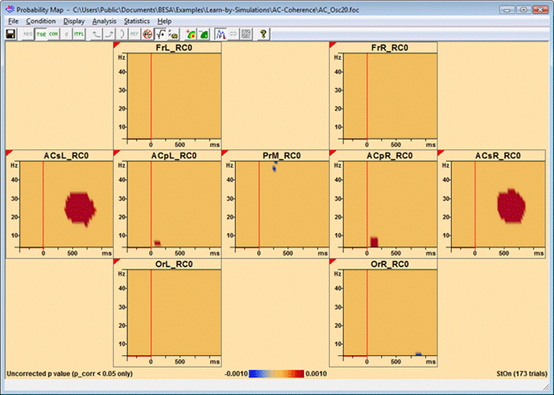
Example for p map of TSE, correction on p=0.05 level. Both significant synchronization and desynchronization is shown (red and blue colors; negative p values indicate desynchronization). The correction yields significant results only at the modelled time-frequency spots, with the exception of the frequency edges in channel PrM, FrR, and the occipital channels. The baseline interval is not tested.
By default, the results are corrected for multiple testing, and only values with a significance of p < 0.05 after correction are kept. Correction can be switched off using statistics options (Statistics/Options from the menu, or use the toolbar button ![]() and select "Options" from the dropdown menu). This Options menu also enables correcting on the significance level p < 0.01. The text at the bottom left of the window indicates that a correction took place to find the significant sampling points, but the remaining p values were not corrected.
and select "Options" from the dropdown menu). This Options menu also enables correcting on the significance level p < 0.01. The text at the bottom left of the window indicates that a correction took place to find the significant sampling points, but the remaining p values were not corrected.
Statistics on Coherence and phase coherence
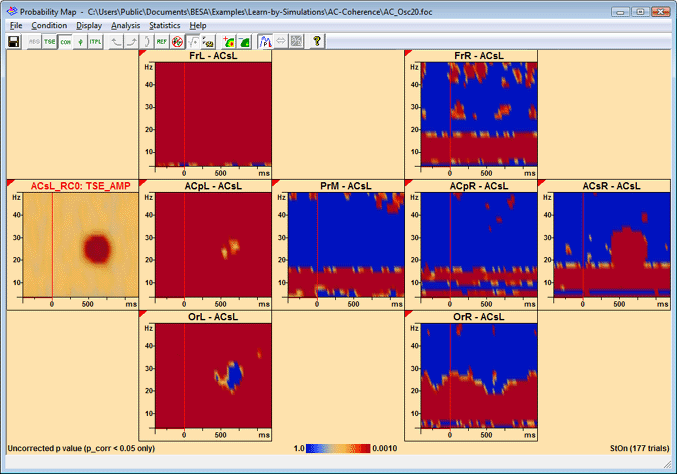
Double-click on a channel (e.g. ACsL) to display its coherence with the other channels. Then press the toolbar button ![]() and select "Current Condition" from the dropdown menu (or select "Statistics/Current Condition" from the menu). This starts the permutation test, which is quite time-consuming. The result looks somewhat like this:
and select "Current Condition" from the dropdown menu (or select "Statistics/Current Condition" from the menu). This starts the permutation test, which is quite time-consuming. The result looks somewhat like this:
Example for the p map of source coherence; correction on p=0.05 level. In all channels, alpha band coherence is significant. Furthermore, significant noise coherence can be observed in the proximate source channels, which only recedes where signal is present which is modelled by the reference channel. The oscillatory coupling between ACsL and ACsR is also significant.
The same procedure applies for a phase coherence analysis. To switch to the p map for phase coherence, simply press the toolbar button ![]() . If statistics mode is already active, the new p map will be computed automatically.
. If statistics mode is already active, the new p map will be computed automatically.
Statistical testing comparing conditions
This example uses the error-related negativity data set in the file 'Examples/TFC-Error-Related Negativity/Correct+Error.foc' (see also BESA Research Tutorial on source coherence on www.besa.de).
After the data file is loaded, start coherence analysis by
- selecting the user montage "ERN9" from the user montages (toolbar button "Usr")
- Loading the paradigm (menu "ERP/Open Paradigm", select paradigm file "Cognitive/ERN.pdg")
- performing an artifact scan (paradigm tab "Artifact", press the "Scan..." button and adjust the amplitude and gradient thresholds to about 180 µV and 75 µV)
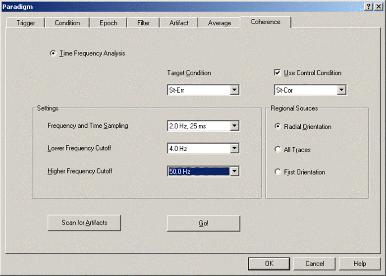
- select the conditions with error and correct response for analysis, triggered on the stimulus (tab "Coherence", select "StErr" as target condition, check the tick mark "Use Control Condition", and select "StCor" as control condition (see figure below). Press the "Go" button. The progress bar is displayed, followed by the temporal-spectral evolution (TSE) display for the target condition.
Settings for comparing conditions in the time-frequency analysis.
Statistics on TSE
Press the ![]() toolbar button to see the difference between target and control condition.
toolbar button to see the difference between target and control condition.
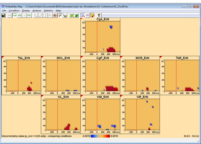
Then press the toolbar button "" and select "Compare Conditions" from the dropdown menu that appears. Alternatively, select "Statistics/Compare Conditions" from the menu. This starts the permutation test. The result looks somewhat like this:
Example of TSE p map when comparing conditions; correction on p=0.05 level. Both significant increase and decrease of TSE in target condition with respect to control condition is shown (red and blue colors; negative p values indicate decrease). The baseline interval is not tested.
As in the case of one condition, the statistics options can be used to switch correction on or off, and to correct on two different significance levels.
Statistics on Coherence and phase coherence
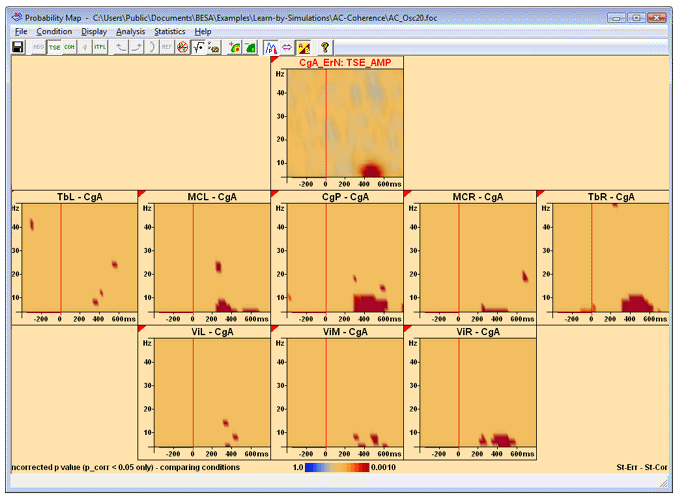
Double-click on a channel (e.g. CgA) to display its coherence with the other channels. Then press the toolbar button ![]() and select "Current Condition" from the dropdown menu (or select "Statistics/Current Condition" from the menu). This starts the permutation test, which is quite time-consuming. The result looks somewhat like this:
and select "Current Condition" from the dropdown menu (or select "Statistics/Current Condition" from the menu). This starts the permutation test, which is quite time-consuming. The result looks somewhat like this:
Example for p-map of coherence comparing conditions; correction on p=0.05 level. The regions where coherence differs significantly between conditions are depicted in red. The main coherent regions are seen in channels CgP and TbR at low frequencies.
Please note that the problems with noise coherence, which arise when testing within one condition, do not arise when comparing conditions. Computation is also much faster, since a different approach is used.
The same procedure applies for a phase coherence analysis. To switch to the p map for phase coherence, simply press the toolbar button ![]() . If statistics mode is already active, the new p map will be computed automatically.
. If statistics mode is already active, the new p map will be computed automatically.
| Review | |
|---|---|
| Source Analysis | |
| Integration with MRI and fMRI | |
| Source Coherence |
|
| Export | |
| MATLAB Interface | |
| Special Topics | |
